Abstract
We present an algorithm to solve the two-dimensional Fredholm integral of the first kind with tensor product structure from a limited number of measurements, with the goal of using this method to speed up nuclear magnetic resonance spectroscopy. This is done by incorporating compressive sensing–type arguments to fill in missing measurements, using a priori knowledge of the structure of the data. In the first step we recover a compressed data matrix from measurements that form a tight frame, and establish that these measurements satisfy the restricted isometry property. Recovery can be done from as few as 10% of the total measurements. In the second and third steps, we solve the zeroth-order regularization minimization problem using the Venkataramanan–Song–Hürlimann algorithm. We demonstrate the performance of this algorithm on simulated data and show that our approach is a realistic approach to speeding up the data acquisition.
Keywords: Fredholm integral, nuclear magnetic resonance, compressive sensing, matrix completion, tight frame
1. Introduction
We present a method of solving the two-dimensional (2D) Fredholm integral of the first kind from a limited number of measurements. This is particularly useful in the field of nuclear magnetic resonance (NMR), in which making a sufficient number of measurements takes several hours. Our work is an extension of the algorithm in [56] based on the new idea of matrix completion; cf. [10, 29, 52].
A 2D Fredholm integral of the first kind is written as
where k1 and k2 are continuous Hilbert–Schmidt kernel functions and f, g ∈ L2(ℝ2); cf. [27]. 2D Fourier, Laplace, and Hankel transforms are all common examples of Fredholm integral equations. Applications of these transformations arise in any number of fields, including methods for solving PDEs [31], image deblurring [4, 38], and moment generating functions [40]. This paper specifically focuses on Laplace-type transforms, where the kernel singular values decay quickly to zero.
To present the main idea of the problem, the data M is measured over sampling times τ1 and τ2 and is related to the object of interest ℱ(x, y) by a 2D Fredholm integral of the first kind with a tensor product kernel,
where ε(τ1, τ2) is assumed to be Gaussian white noise. In most applications, including NMR, the kernels k1 and k2 are explicit functions that are known to be smooth and continuous a priori. Solving a Fredholm integral with smooth kernels is an ill-conditioned problem, since the kernel’s singular values decay quickly to zero [34]. This makes the problem particularly interesting, as small variations in the data can lead to large fluctuations in the solution.
For our purposes, ℱ(x, y) represents the joint probability density function of the variables x and y. Specifically in NMR, x and y can be the measurements of the two combination of the longitudinal relaxation time T1, transverse relaxation time T2, diffusion D, and other dynamic properties. Knowledge of the correlation of these properties of a sample is used to identify its microstructure properties and dynamics [6].
This paper focuses on the discretized version of the 2D Fredholm integral,
| (1.1) |
where our data is the matrix M ∈ ℝN1×N2, matrices K1 ∈ ℝN1×Nx and K2 ∈ ℝN2×Ny are discretized versions of the smooth kernels k1 and k2, and the matrix F ∈ ℝNx×Ny is the discretized version of the probability density function ℱ(x, y) which we are interested in recovering. We also assume that each element of the Gaussian noise matrix E has zero mean and constant variance. And since we have assumed that ℱ(x, y) is a joint probability density function, each element of F is nonnegative.
Venkataramanan, Song, and Hürlimann [56] laid out an efficient strategy for solving this problem given complete knowledge of the data matrix M. The approach centers around finding an intelligent way to solve the Tikhonov regularization problem,
| (1.2) |
where || · ||F is the Frobenius norm.
There are three steps to the algorithm in [56] for solving (1.2).
-
Compress the data. Let the SVD of Ki be
Because K1 and K2 are sampled from smooth functions k1 and k2, the singular values decay quickly to 0. Let s1 be the number of nonzero singular values of K1, and let s2 be the number of nonzero singular values of K2. Then Ui ∈ ℝNi×si and Si ∈ ℝsi×si for i = 1, 2, as well as V1 ∈ ℝNx×s1 and V2 ∈ ℝNy×s2.
The data matrix M can be projected onto the column space of K1 and the row space of K2 by . We denote this as . The Tikhonov regularization problem (1.2) is now rewritten as(1.3) (1.4) where (1.4) comes from U1 and U2 having orthogonal columns, and the second and third terms in (1.3) being independent of F. The key note here is that M̃ ∈ ℝs1×s2, which significantly reduces the complexity of the computations.
Optimization. For a given value of α, (1.4) has a unique solution due to the second term being quadratic. We shall detail the method of finding this solution in section 4.
Choosing α. Once (1.4) has been solved for a specific α, an update for α is chosen based on the characteristics of the solution in step 2. Repeat steps 2 and 3 until convergence. Again, this is detailed in section 4.
The approach in [56] assumes complete knowledge of the data matrix M. However, in applications with NMR, there is a cost associated with collecting all the elements of M, namely, time. With the microstructure-related information contained in the multidimensional diffusion-relaxation correlation spectrum of the biological sample [49, 22, 25, 20, 35, 54] and high-resolution spatial information that magnetic resonance imaging (MRI) techniques can provide, there is a need to combine the multidimensional correlation spectra NMR with 2D/3D MRI for preclinical and clinical applications [21]. Without any acceleration, however, it could take several days to acquire this data.
In practice, the potential pulse sequences for the combined multidimensional diffusion-relaxation MRI would be single spin echo (90°–180° acquisition and spatial localization) with saturation, inversion recovery, driven-equilibrium preparation to measure T1-T2 correlation, and diffusion weighting preparation for D-T2 measurements. With these MRI pulse sequences, a single point in the 2D T1-T2 or D-T2 space is acquired for each “shot,” and the total time for the sampling of the T1-T2 or D-T2 space is determined directly by the number of measurements required to recover F from (1.2). A vastly reduced number of sample points in M, together with rapid MRI acquisition techniques, which can include, e.g., parallel imaging [50], echo planar imaging (EPI) [24], gradient-recalled echo [36], and sparse sampling with compressed sensing [45], could reduce the total experiment time sufficiently to make this promising technique practicable for preclinical and clinical in vivo studies.
Notice that, despite collecting all N1 × N2 data points in M, step 1 of the algorithm immediately throws away a large amount of that information, reducing the number of data points to a matrix of size s1 × s2. M̃ is effectively a compressed version of the original M, containing the same information in a smaller number of entries. But this raises the question of why all of M must be collected when a large amount of information is immediately thrown away, since we are interested only in M̃.
This question is what motivates the introduction of a compressive sensing–type approach. The task is to undersample signals that are “compressible,” meaning that the signal is sparse in some basis representation [12, 11, 23]. The problem of recovering M falls into a subset of this field known as low-rank matrix completion; see [10, 29, 14].
An n × n matrix X that is rank r requires approximately nr parameters to be completely specified. If r ≪ n, then X is seen as being compressible, as the number of parameters needed to specify it is much less than its n2 entries. It is less clear how to recover X from a limited number of coefficients efficiently. But the results of [10] showed that it is possible to recover X from, up to a constant, nr log(n) measurements by employing a simple optimization problem. These findings were inspired, at least in part, by [12, 11]. Also, the types of measurements we utilize in this paper, operator bases with bounded norm, originated via quantum state tomography [30].
Compressive sensing has been used in various forms of medical imaging for several years. The authors of [45] originally proposed speeding up MRI acquisition. The authors of [47] introduced group sparsity into consideration for accelerating T2-weighted MR. Finally, the authors of [55, 39] both introduced basic ideas of compressive sensing into the NMR framework and attained promising results, but the results did not utilize the matrix completion aspect of the physical problem and did not introduce any theoretical guarantees for reconstruction.
This paper develops an alternative to [56] which incorporates matrix completion in order to recover M̃ from significantly fewer measurements. It is organized as follows. Section 2 examines how recovery of M̃ fits into existing theory and shows that data from the 2D Fredholm integral can be recovered from 10% of the measurements. Section 3 covers the practical considerations of the problem and discusses the error created by our reconstruction. Section 4 covers the algorithms used to solve the low-rank minimization problem and invert the 2D Fredholm integral to obtain F. Section 5 shows the effectiveness of this reconstruction on simulated data. Appendix A contains a detailed proof of the central theorem of this paper.
2. Data recovery using matrix completion
2.1. Background for matrix completion
The problem of matrix completion has been in the center of scientific interest and activity in recent years [10, 26, 29, 51, 5, 9, 13, 7]. The basic problem revolves around trying to recover a matrix X0 ∈ ℝn1×n2 from only a fraction of the N1 × N2 measurements required to observe each element of M. Without any additional assumptions, this is an ill-posed problem. However, there have been a number of attempts to add natural assumptions to make this problem well-posed. Other than assuming that X0 is low rank, as we mentioned in section 1, there are assumptions that X0 is positive definite [28, 42], or that X0 is a distance matrix [2], or that X0 has a nonnegative factorization [57]. A survey of some of these other methods can be found in [37].
For our purposes, we shall focus on low-rank matrix completion, as that is the most natural. Let X0 be rank r. Consider a linear operator 𝒜: ℝn1×n2 → ℝm. Then our observations take the form
| (2.1) |
where z represents a noise vector that is typically white noise, though not necessarily.
The naive way to proceed would be to solve the nonlinear optimization problem
| (2.2) |
However, the objective function rank(Z) makes the problem NP-hard. So instead we define the convex envelope of the rank function.
Definition 2.1
Let σi(X) be the ith singular value of a rank r matrix X. Then the nuclear norm of X is
We now proceed by attempting to solve the convex relaxation of (2.2),
| (2.3) |
As with traditional compressive sensing, there exists a restricted isometry property (RIP) over the set of matrices of rank r.
Definition 2.2
A linear operator 𝒜: ℝn1×n2 → ℝm satisfies the RIP of rank r with isometry constant δr if, for all rank r matrices X,
The RIP has been shown to be a sufficient condition for solving (2.3) [52, 8, 26]. These papers build on each other to establish the following theorem.
Theorem 2.3
Let X0 be an arbitrary matrix in ℂm×n. Assume that δ5r < 1/10. Then the X̂ obtained from solving (2.3) obeys
| (2.4) |
where X0,r is the best r rank approximation to X0, and C0,C1 are small constants depending only on the isometry constant.
This means that, if the measurement operator 𝒜 satisfies RIP, then reconstruction via convex optimization behaves stably in the presence of noise. This result is very important in the context of the 2D Fredholm problem, as inversion of the Fredholm integral is very sensitive to noise. The bound in (2.4) guarantees that our reconstructed data behaves stably and will not create excess noise that would cause issues in the inversion process.
2.2. Matrix completion applied to NMR
For the NMR problem, let us say that
| (2.5) |
where Ui ∈ ℝNi×si, M̃ ∈ ℝs1×s2, and E ∈ ℝN1×N2. This means that
| (2.6) |
To subsample the data matrix M, we shall observe it on random entries. Let Ω ⊂ {1, …, N1} × {1, …, N2} be the set of indices where we observe M. For |Ω| = m, let the indices be ordered as . Then we define the masking operator 𝒜Ω as
Recall that the goal is to recover M̃0. This means that our actual sampling operator is
Now the problem of speeding up NMR can be written as an attempt to recover M̃0 from measurements
| (2.7) |
Note that [56] is assuming Ω = {1, …, N1} × {1, …, N2}, making the sampling operator .
Then in the notation of this NMR problem, our recovery step takes the form
| (2.8) |
Now the key question becomes whether ℛΩ satisfies the RIP. As we said in section 2.1, the RIP is a sufficient condition for an operator to satisfy the noise bounds of Theorem 2.3. Without this, there is no guarantee that solving (2.8) yields an accurate prediction of M̃. For this reason, the rest of this section shall focus on proving that ℛΩ is an RIP operator.
First, we must define the notion of a Parseval tight frame.
Definition 2.4
A Parseval tight frame for a d-dimensional Hilbert space ℋ is a collection of elements {ϕj}j∈J ⊂ ℋ for an index set J such that
This automatically forces |J| ≥ d.
This definition is very closely related to the idea of an orthonormal basis. In fact, if |J| = d, then {ϕj}j∈J would be an orthonormal basis. This definition can be thought of as a generalization. Frames have the benefit of giving overcomplete representations of the function f, making them much more robust to errors and erasures than orthonormal bases [17, 41, 15]. This redundancy is exactly what we will be taking advantage of in Theorem 2.6.
Further, we introduce a definition used in [29].
Definition 2.5
A bounded norm Parseval tight frame with incoherence μ is a Parseval tight frame {ϕj}j∈J on ℂd×d that also satisfies
| (2.9) |
The paper [29] defines this type of bound on an orthonormal basis. Note that, in the case of {ϕj}j∈J being an orthonormal basis, |J| = d2, reducing the bound in (2.9) to ||ϕj||2 ≤ μ/d, as in the case of [29].
Now notice that in our problem, ignoring noise, each observation can be written as
where (resp., ) is the jth row of U1 (resp., U2). Noting that U1 and U2 are left orthogonal (i.e., ), one can immediately show that forms a Parseval tight frame for ℝs1×s2. Also, because K1 and K2 are discretized versions of smooth continuous functions, { } are a bounded norm frame for a reasonable constant μ (see further discussion of μ in section 3.2). Thus, ℛΩ is generated by randomly selecting measurements from a bounded norm Parseval tight frame.
We now have the necessary notation to state our central theorem, which establishes bounds on the quality of reconstruction from (2.8) in the presence of noise. The theorem and proof rely on a generalization of [44], which only assumes the measurements to be orthonormal basis elements.
It is interesting to note that, because our measurements are overcomplete (|J| > s1s2), our system of equations is not necessarily underdetermined. However, Theorem 2.6 still gives guarantees on how the reconstruction scales with the noise, regardless of this detail. This is a difference from most compressive sensing literature. Generally the goal is to show that an underdetermined system has a stable solution. In our case we are showing that, regardless of whether or not the system is underdetermined, our reconstruction is stable in the presence of noise and the reconstruction error decreases monotonically with the number of measurements.
Theorem 2.6
Let {ϕj}j∈J ⊂ ℂs1×s2 be a bounded norm Parseval tight frame, with incoherence parameter μ. Let n = max(s1, s2), and let the number of measurements m satisfy
where C is a constant. Let the sampling operator ℛΩ be defined for Ω ⊂ J, with Ω = {i1, …, im}, as
Let measurements y satisfy (2.7). Then, with probability greater than 1−e−Cδ2 over the choice of Ω, the solution M̃ to (2.8) satisfies
| (2.10) |
where .
To prove this result, we need a key lemma, which establishes that our measurements satisfy the RIP.
Lemma 2.7
Let {ϕj}j∈J ⊂ ℂs1×s2 be a bounded norm Parseval tight frame, with incoherence parameter μ. Fix some 0 < δ < 1. Let n = max(s1, s2), and let the number of measurements m satisfy
| (2.11) |
where C ∝ 1/δ2. Let the sampling operator ℛΩ be defined for Ω ⊂ J, with Ω = {i1, …, im}, as
Then, with probability greater than 1 − e−Cδ2 over the choice of Ω, satisfies the RIP of rank r with isometry constant δ.
The proof of this lemma is found in Appendix A and follows [44], where the claim is proved for an orthonormal basis. The main point here is to generalize the measurements to a bounded norm Parseval tight frame (also mentioned in [48], however, not considering when m > n2).
Proof of Theorem 2.6
We assume that Lemma 2.7 is true. Lemma 2.7 states that satisfies the RIP. However, (2.8) is stated using only ℛΩ as the measurement operator.
This means we must include a scaling factor of to understand the noise bound. Let be the percentage of elements observed. Then, to utilize the RIP, we must try to solve the problem
| (2.12) |
While scaling by a constant does not affect the result of the minimization problem, it does help us better understand the error in our reconstruction.
Theorem 2.3 tells us that our reconstruction error is bounded by a constant multiple of the error bound. But (2.12) means we can rewrite the error bound as
thus attaining the desired inequality.
Remark 1
Examination of the proof of Lemma 2.7 shows that the bound on m in (2.11) is actually not sharp. If one refers to (A.1) in Appendix A, m is actually bounded below by a factor of logm. In (A.2) we simply overestimate this term with log |J| for simplicity. However, in reality the bound is
Let N = Cλμrn log5 n. This would give the bound m ≥ e−W−1(−1/N), where W−1 is the lower branch of the Lambert W function [19]. Taking the first three terms of a series approximation of W−1 in terms of log(1/N) and log(log(N)) [18] gives us
| (2.13) |
Note that taking three terms is sufficient as each subsequent term is asymptotically small compared to the previous. The bound in (2.13) is clearly much more intricate than simply bounding by m ≥ Cλμrn log5 n log |J|, but for typical sizes of |J| in the Fredholm integral setting, this results in m decreasing by less than 5% from its original size.
3. Numerical considerations
Section 2 gives theoretical guarantees about the error of estimating M̃0 with the recovered M̃. We shall address several issues related to practical applications in this section. We shall let M̃0 be the original compressed data matrix we are hoping to recover, and let M̃ be the approximation obtained by solving (2.8) for the sampling operator ℛΩ. We consider the guarantee given in (2.4) term by term.
For the rest of this paper, we take the kernels K1 and K2 to be Laplace-type kernels with quickly decaying singular values. For our purposes, we shall use the kernels k1(τ1, x) = 1 − e−τ1/x and k2(τ2, y) = e−τ2/y to represent the general data structure of most multiexponential NMR spectroscopy measurements. The same kernels shall be used in section 5 for simulations and experiments. Also, τ1 is logarithmically sampled between 0.0005 and 4, and τ2 is linearly sampled between 0.0002 and 0.4, as these are typical values in practice. Also for this section, F is taken to be a two-peak distribution, namely Model 3 from section 5.
When needed, we set s1 = s2 = 20. This choice is determined by the discrete Picard condition (DPC) [33]. For ill-conditioned kernel problems Kf = g, with {ui} denoting left singular vectors of K and {σi} the corresponding singular values, the DPC guarantees that the best reconstruction of f is given by keeping all σi ≠ 0 such that on average decays to zero as σi decrease. For our kernels with tensor product structure in (1.1), Figure 1 shows the relevant singular values and vectors to keep. The s1 = s2 = 20 rectangle provides a close estimate for what fits inside this curve, implying that at a minimum we could set s1 = s2 = 20 to satisfy the DPC. The DPC provides a stronger condition than simply keeping the largest singular values or attempting to preserve some large percentage of the energy [32].
Figure 1.
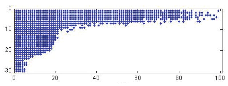
Points denote which singular values of K1 (rows of plot) and K2 (columns of plot) to keep in order to satisfy the DPC for stable inversion.
3.1. Noise bound in practice
Theorem 2.3 hinges on the assumption that δ5r < 1/10, where δr is the isometry constant for rank r. This puts a constraint on the maximum size of r. Let us denote that maximal rank by r0. If we knew a priori that M̃0 was at most rank r0, then this term of would have zero contribution, as M̃0 = M̃0,r. However, because of (2.6), M̃0 could theoretically be full rank, since S1 and S2 are decaying but not necessarily 0.
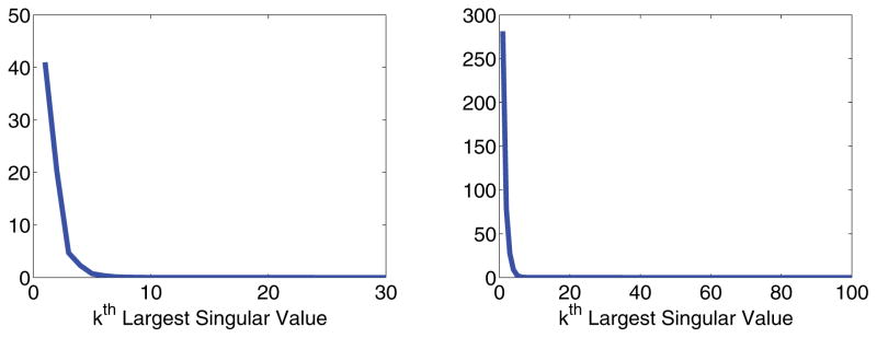
This problem is rectified by utilizing the knowledge that K1 and K2 have rapidly decaying singular values. Figure 2 shows just how rapidly the singular values decay for a typical choice of kernels and discretization points. This means M̃0 from (2.6) must have even more rapidly decaying singular values, as is multiplied by both S1 and S2. Figure 3 shows that the singular values of M̃0 drop to zero almost immediately for a typical compressed data matrix.
Figure 2.
Plots of the singular value decay of the kernels. Left: K1. Right: K2.
Figure 3.
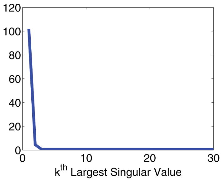
Plot of the singular value decay for data matrix M.
This means that even for small r0, is very close to zero, as the tail singular values of M̃0 are almost exactly zero.
Figure 4 shows how the relative error decays for larger percentages of measurement, and how that curve matches the predicted curve of p−1/2||e||2. One can see from this curve that the rank r error does not play any significant role in the reconstruction error.
Figure 4.
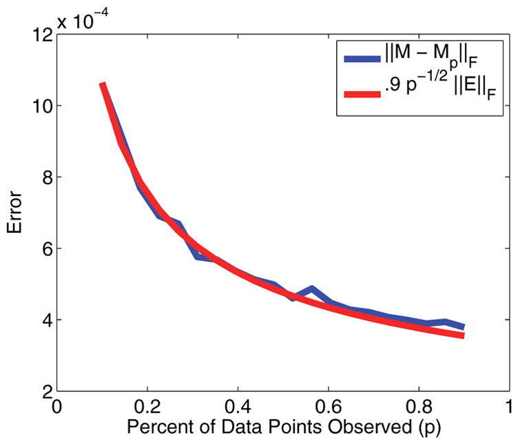
Plot of the error in reconstruction.
3.2. Incoherence
The incoherence parameter μ to bound the number of measurements in (2.11) plays a vital role in determining m in practice. It determines whether the measurements { } are viable for reconstruction from significantly reduced m, even though they form a Parseval tight frame.
To show that μ does not make reconstruction prohibitive, we demonstrate on a typical example of K1 and K2, as described at the beginning of this section.
Figure 5 shows the for each measurement { } from the above description, making . While this bound on μ is not ideal, as it makes m > n2, there are two important points to consider. First, as was mentioned in section 2.2, Theorem2.3 guarantees strong error bounds regardless of the system being underdetermined. Second, as is shown in section 3.3, the estimate M̃ is still significantly better than a simple least squares minimization, which in theory applies as the system isn’t underdetermined.
Figure 5.
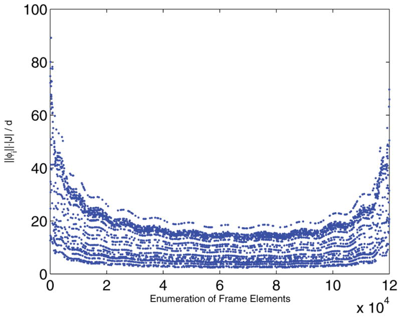
Plot of for each measurement element from the NMR problem.
Also note from Figure 5 the fact that and differ greatly from . This implies that, while a small number of the entries are somewhat problematic and coherent with the elementary basis, the vast majority of terms are perfectly incoherent. This implies that Theorem 2.3 is a nonoptimal lower bound on m. Future work will be to examine the possibility of bounding m below with an average or median coherence, or considering a reweighted nuclear norm sampling similar to [16]. Another possibility is to examine the idea of asymptotic incoherence [1].
3.3. Least squares comparison
One could also attempt to solve for M̃0 using a least squares algorithm on the observed measurements via the Moore–Penrose pseudoinverse. However, as we shall show, due to noise and ill-conditioning, this is not a viable alternative to the nuclear norm minimization algorithm employed throughout this paper. As an example, we shall again use K1 and K2 as described in the beginning of this section. The noise shall range over various signal-to-noise ratios (SNRs).
We will consider a noisy estimate M̃ of the compressed matrix M̃0, generated through the pseudoinverse, nuclear norm minimization, or simply the projection of a full set of measurements M via . Figure 6 shows the relative error of each of these recoveries, defining error to be
Figure 6.
Relative error of least squares approximation compared to nuclear norm minimization versus percentage of measurements kept. Left: SNR = 15dB. Center: SNR = 25dB. Right: SNR = 35dB.
Clearly, nuclear norm minimization, even for a small fraction of measurements kept, mirrors the full measurement compression almost perfectly, as was shown in Figure 4. However, the least squares minimization error is drastically higher. Even at 20% measurements kept, the difference in error between least squares reconstruction and the full measurement projection error is 4 times higher than the difference between nuclear norm reconstruction and the full measurement projection error.
4. Algorithm
The algorithm for solving for F in (1.1) from partial data consists of three steps. An overview of the original algorithm in [56] is in section 1. Our modification and the specifics of each step are detailed below.
-
Construct M̃ from given measurements. Let y = ℛΩ(M̃0) + e be the set of observed measurements, as in (2.7). Even though section 2 makes guarantees for solving (2.8), we can instead solve the relaxed Lagrangian form
(4.1) To solve (4.1), we use the singular value thresholding algorithm from [5, 46]. To do this, we need some notation. Let the matrix derivative of the L2 norm term be written asWe also need the singular value thresholding operator 𝒮ν that reduces each singular value of some matrix X by ν. In other words, if the SVD of X = UΣV′, thenUsing this notation, the algorithm can then be written as a simple, two-step iterative process. Choose a τ > 0. Then, for any initial condition, solve the iterative process(4.2) The choices of τ and μ are detailed in [46], along with adaptations of this method that speed up convergence. However, this method is guaranteed to converge to the correct solution.
This means that, given partial observations y, the iteration scheme in (4.2) converges to a matrix M̃, which is a good approximation of M̃ +0. Once M̃ has been generated, we recover F by solving(4.3) -
Optimization. For a given value of α, (4.3) has a unique solution due to the second term being quadratic. This constrained optimization problem is then mapped onto an unconstrained optimization problem for estimating a vector c.
Let f be the vectorized version of F and m be a vectorized version of M̃. Then we define the vector c from f implicitly byHere, ⊗ denotes the Kronecker product of two matrices. This definition of c comes from the constraint that F ≥ 0 in (4.3), which can now be reformed as the unconstrained minimization problem(4.4) whereand H(x) is the Heaviside function. Also, Ki,· denotes the ith row of K. The optimization problem (4.4) is solved using a simple gradient descent algorithm.
-
Choosing α. There are several methods for choosing the optimal value of α.
-
Butler–Reeds–Dawson (BRD) method. Once an iteration of step 2 has been completed, it is shown in [56] that a better value of α can be calculated by
If one iterates between step 2 and the BRD method, the value of α converges to an optimal value. This method is very fast; however, it can have convergence issues in the presence of large amounts of noise, as well as on real data [53].
-
S-curve. Let Fα be the value returned from step 2 for a fixed α. The choice of α should be large enough that Fα is not being overfitted and unstable to noise, yet small enough that Fα actually matches reality. This is done by examining the “fit error”
This is effectively calculating the standard deviation of the resulting reconstruction. Plotting χ(α) for various values of α generates an S-curve, as shown in Figure 7. The interesting value of α occurs at the bottom “heel” of the curve (i.e., ). This is because, at αheel, the fit error is no longer demonstrating overfitting as it is to the left of αheel, yet is still matching the original data, unlike to the right of αheel. This method is slower than the BRD method; however, it is usually more stable in the presence of noise.
-
Figure 7.
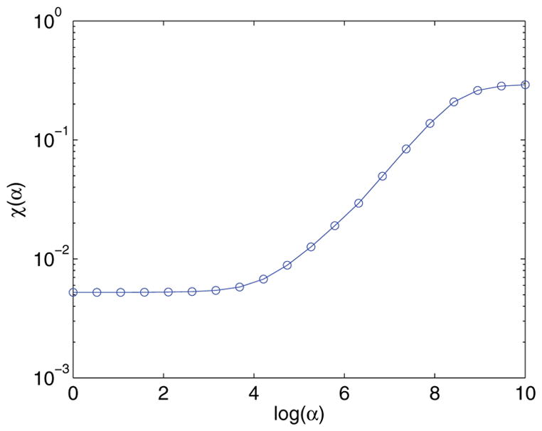
Plot of the fit error for various α.
For the rest of this paper, we use the S-curve method of choosing α.
5. Simulation results
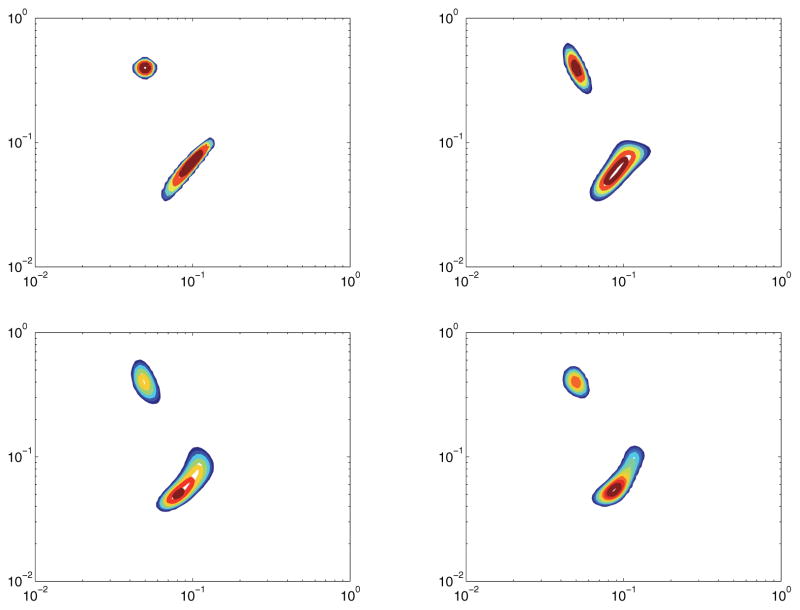
In our simulations, we shall use the kernels k1(τ1, x) = 1 − e−τ1/x and k2(τ2, y) = e−τ2/y and sample τ1 logarithmically and τ2 linearly, as was done in section 3. Our simulations revolve around inverting subsampled simulated data to recover the density function F(x, y). We shall test three models of F(x, y). In Model 1, F(x, y) is a small variance Gaussian. In Model 2, F(x, y) is a positively correlated density function. In Model 3, F(x, y) is a two-peak density, one peak being a small circular Gaussian and the other being a ridge with positive correlation.
The data is generated for a model of F(x, y) by discretizing F and computing
where E is Gaussian noise. That data is then randomly subsampled by keeping only a λ fraction of the entries.
Each true model density F(x, y) is sampled logarithmically in x and y. τ1 is logarithmically sampled N1 = 30 times, and τ2 is linearly sampled N2 = 4000 times. Each model is examined for various SNRs and values of λ, and α is chosen using the S-curve approach for each trial.
Let us also define the signal-to-noise ratio (SNR) for our data to be
Note that [56] has extensively examined steps 2 and 3 of this algorithm, including the effects of α and the SNR on the reconstruction of F. Our examination focuses on the differences between the F generated from full knowledge of the data and the F generated from subsampled data. For this reason, Ffull refers to the correlation spectrum generated from full knowledge of the data using the algorithm from [56]. Fλ refers to the correlation spectrum generated from only a λ fraction of the measurements using our algorithm.
5.1. Model 1
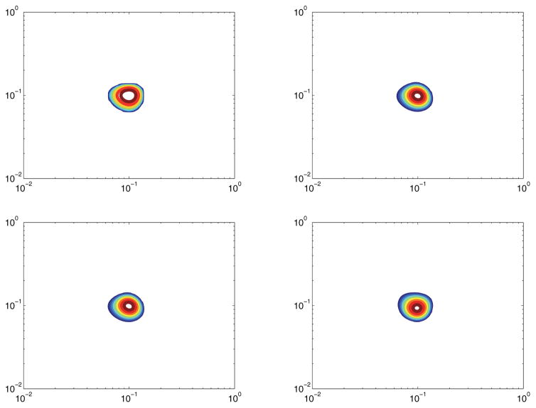
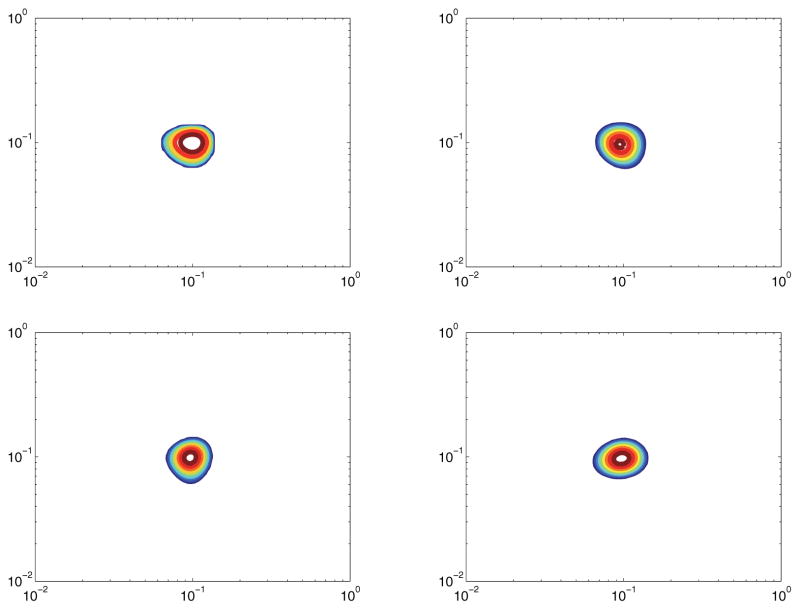
In this model, F(x, y) is a small variance Gaussian. This is the simplest example of a correlation spectrum, given that the dimensions are uncorrelated. F(x, y) is centered at (x, y) = (.1, .1) and has standard deviation .02. The maximum signal amplitude is normalized to 1. This model of F(x, y) is a base case for any algorithm. In other words, any legitimate algorithm for inverting the 2D Fredholm integral must at a minimum be successful in this case.
Figure 8 shows the quality of reconstruction of a simple spectrum with an SNR of 30dB. Figure 9 shows the same spectrum, but with an SNR of 15dB. Almost nothing is lost in either reconstruction, implying that both the original algorithm and our compressive sensing algorithm are very robust to noise for this simple spectrum.
Figure 8.
Model 1 with SNR of 30dB. Top left: True spectrum. Top right: Ffull. Bottom left: Reconstruction from 30% measurements. Bottom right: Reconstruction from 10% measurements.
Figure 9.
Model 1 with SNR of 15dB. Top left: True spectrum. Top right: Ffull. Bottom left: Reconstruction from 30% measurements. Bottom right: Reconstruction from 10% measurements.
5.2. Model 2
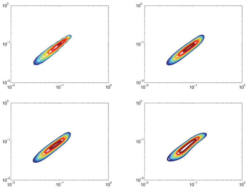
In this model, F(x, y) is a positively correlated density function. The spectrum has a positive correlation, thus creating a ridge through the space. F(x, y) is centered at (x, y) = (.1, .1), with the variance in the x + y direction being 7 times greater than the variance in the x − y direction. The maximum signal amplitude is normalized to 1. This is an example of a spectrum where it is essential to consider the 2D image. A projection onto one dimension would yield an incomplete understanding of the spectrum, as neither the T1 projection nor the T2 projection would convey that the ridge is very thin. This is a more practical test of our inversion algorithm.
Figure 10 shows the quality of reconstruction of a correlated spectrum with an SNR of 30dB. Figure 11 shows the same spectrum, but with an SNR of 20dB. There is slight degradation in the 10% reconstruction, but the reconstructed spectrum is still incredibly close to Ffull. Overall, both of these figures show the quality of our compressive sensing reconstruction relative to using the full data.
Figure 10.
Model 2 with SNR of 30dB. Top left: True spectrum. Top right: Ffull. Bottom left: Reconstruction from 30% measurements. Bottom right: Reconstruction from 10% measurements.
Figure 11.
Model 2 with SNR of 20dB. Top left: True spectrum. Top right: Ffull. Bottom left: Reconstruction from 30% measurements. Bottom right: Reconstruction from 10% measurements.
5.3. Model 3
In this model, F(x, y) is a two-peak density, with one peak being a small circular Gaussian and the other being a ridge with positive correlation. The ridge is centered at (x, y) = (.1, .1), with the variance in the x + y direction being 7 times greater than the variance in the x − y direction. The circular part is centered at (x, y) = (.05, .4). The maximum signal amplitude is normalized to 1. This is an example of a common, complicated spectrum that occurs during experimentation.
Figure 12 shows the quality of reconstruction of a two-peak spectrum with an SNR of 35dB. In this instance, there is some degradation from Ffull to any of the reconstructed data sets. Once again, there is slight degradation in the 10% model, but the compressive sensing reconstructions are still very close matches to Ffull.
Figure 12.
Model 3 with SNR of 30dB. Top left: True spectrum. Top right: Ffull. Bottom left: Reconstruction from 30% measurements. Bottom right: Reconstruction from 10% measurements.
6. Conclusion
In this paper, we introduce a matrix completion framework for solving 2D Fredholm integrals. This method allows us to invert the discretized transformation via Tikhonov regularization using far fewer measurements than previous algorithms. We proved that the nuclear norm minimization reconstruction of the measurements is stable and computationally efficient, and demonstrated that the resulting estimate of ℱ(x, y) is consistent with using the full set of measurements. This allows us in application to reduce the measurements conducted by a factor of 5 or more.
While the theoretical framework of this paper applies to 2D NMR spectroscopy, the approach is easily generalized to larger-dimensional measurements. This allows for accelerated acquisition of 3D correlation maps [3] that would otherwise take days to collect. This shall be a subject of forthcoming work.
Acknowledgments
The authors would like to thank Dr. Richard Spencer for helpful discussions, and the anonymous reviewers for their constructive comments.
Appendix A. Proof of Lemma 2.7
Let us define
Note that the set of all rank r matrices in ℂs1×s2 is a subset of U by Hölder’s inequality. For the proof, we need some notation:
The RIP can be rewritten as
which is implied by
So we need to show that εr(𝒜) ≤ 2δ − δ2 ≡ ε.
One can then define a norm on the set of all self-adjoint operators from ℂs1×s2 to ℂs1×s2 by
The proof that this is a norm, and that the set of self-adjoint operators is a Banach space with respect to ||·||(r), is found in [44].
We can now write εr(𝒜) = ||𝒜 * 𝒜 − ℐ||(r). For our purposes, as with most compressive sensing proofs, we first bound 𝔼εr(𝒜) and then show that εr(𝒜) is concentrated around its mean.
For our problem of dealing with tight frame measurements, let , where . Also, let be independent copies of the random variable χi. Finally, let εi be a random variable that takes values ±1 with equal probability. Then we have that
Now we cite Lemma 3.1 of [44], which is general enough to remain unchanged in the case of tight frames.
Lemma A.1
Let have a uniformly bounded norm, ||Vi|| ≤ K. Let n = max(s1, s2), and let be independent and identically distributed uniform ±1 random variables. Then
where and C0 is a universal constant.
For our purposes, . Then
Here,
| (A.1) |
If we take E0 = 𝔼εr(𝒜) and , then (A.1) gives us
Fix some λ ≥ 1, and choose
| (A.2) |
This makes .
The next step is to show that εr(𝒜) does not deviate far from 𝔼εr(𝒜). Let 𝒜 * 𝒜 − ℐ = χ be a random variable and χ′ be an independent copy of χ. We now note that
Define , so that . Clearly
We now use the following result by Ledoux and Talagrand in [43].
Theorem A.2
Let be independent symmetric random variables on some Banach space such that ||𝒴i|| ≤ R. Let . Then for any integers l ≥ q and any t > 0
where K is a universal constant.
Now for appropriate choices of q, l, and t, and with an appropriate λ such that λ ≥ A/ε2 for some constant A, we get that
where C is a constant. Thus, the probability of failure is exponentially small in λ.
Footnotes
This work was performed by an employee of the U.S. Government or under U.S. Government contract. The U.S. Government retains a nonexclusive, royalty-free license to publish or reproduce the published form of this contribution, or allow others to do so, for U.S. Government purposes. Copyright is owned by SIAM to the extent not limited by these rights.
Contributor Information
Alexander Cloninger, Email: alex@math.umd.edu.
Wojciech Czaja, Email: wojtek@math.umd.edu.
Ruiliang Bai, Email: ruiliang.bai@nih.gov.
Peter J. Basser, Email: pjbasser@helix.nih.gov.
References
- 1.Adcock B, Hansen AC, Poon C, Roman B. Breaking the Coherence Barrier: Asymptotic Incoherence and Asymptotic Sparsity in Compressed Sensing. 2013 preprint, arXiv:1302.0561v1 [cs.IT] [Google Scholar]
- 2.Alfakih AY, Khandani A, Wolkowicz H. Solving Euclidean distance matrix completion problems via semidefinite programming. Comput Optim Appl. 12(1998):13–30. [Google Scholar]
- 3.Arns CH, Washburn KE, Callaghan PT. Multidimensional NMR Inverse Laplace Spectroscopy in Petrophysics. Petrophys. 48(2007):380–392. [Google Scholar]
- 4.Bonettini S, Zanella R, Zanni L. A scaled gradient projection method for constrained image deblurring. Inverse Problems. 25(2009):015002. [Google Scholar]
- 5.Cai JF, Candès EJ, Shen Z. A singular value thresholding algorithm for matrix completion. SIAM J Optim. 20(2010):1956–1982. [Google Scholar]
- 6.Callaghan PT, Arns CH, Galvosas P, Hunter MW, Qiao Y, Washburn KE. Recent Fourier and Laplace perspectives for multidimensional NMR in porous media. Magn Reson Imaging. 25(2007):441–444. doi: 10.1016/j.mri.2007.01.114. [DOI] [PubMed] [Google Scholar]
- 7.Candès E, Eldar YC, Strohmer T, Voroninski V. Phase retrieval via matrix completion. SIAM J Imaging Sci. 6(2013):199–225. [Google Scholar]
- 8.Candès EJ, Plan Y. Tight oracle bounds for low-rank matrix recovery from a minimal number of random measurements. IEEE Trans Inform Theory. 57(2009):2342–2359. [Google Scholar]
- 9.Candès E, Plan Y. Matrix completion with noise. Proc IEEE. 98(2010):925–936. [Google Scholar]
- 10.Candès E, Recht B. Exact matrix completion via convex optimization. Found Comput Math. 9(2008):717–772. [Google Scholar]
- 11.Candès E, Romberg J. Sparsity and incoherence in compressive sampling. Inverse Problems. 23(2007):969–985. [Google Scholar]
- 12.Candès E, Romberg J, Tao T. Robust uncertainty principles: Exact signal reconstruction from highly incomplete frequency information. IEEE Trans Inform Theory. 52(2006):489–509. [Google Scholar]
- 13.Candès E, Strohmer T, Voroninski V. PhaseLift: Exact and stable signal recovery from magnitude measurements via convex programming. Comm Pure Appl Math. 66(2012):1241– 1274. [Google Scholar]
- 14.Candès E, Tao T. The power of convex relaxation: Near-optimal matrix completion. IEEE Trans Inform Theory. 56(2010):2053–2080. [Google Scholar]
- 15.Casazza PG, Fickus M, Kovǎcevíc J, Leon MT, Tremain JC. A physical interpretation of tight frames. In: Heil C, editor. Harmonic Analysis and Applications, Appl. Numer. Harmon. Anal. Birkhäuser Boston; Boston: 2006. pp. 51–76. [Google Scholar]
- 16.Chen Y, Bhojanapalli S, Sanghavi S, Ward R. Coherent Matrix Completion. 2013 preprint, arXiv:1306.2979v2 [stat.ML] [Google Scholar]
- 17.Christensen O. An Introduction to Frames and Riesz Bases. Birkhäuser Boston; Boston: 2003. [Google Scholar]
- 18.Comtet L. Advanced Combinatorics. Reidel; Dordrecht, The Netherlands: 1974. [Google Scholar]
- 19.Corless RM, Gonnet GH, Hare DEG, Jeffrey DJ, Knuth DE. On the Lambert W function. Adv Comput Math. 5(1996):329–359. [Google Scholar]
- 20.Deoni SC, Rutt BK, Arun T, Pierpaoli C, Jones DK. Gleaning multicomponent T1 and T2 information from steady-state imaging data. Magn Reson Med. 60(2008):1372–1387. doi: 10.1002/mrm.21704. [DOI] [PubMed] [Google Scholar]
- 21.Deoni SC, Rutt BK, Peters TM. Rapid combined T1 and T2 mapping using gradient recalled acquisition in the steady state. Magn Reson Med. 49(2003):515–526. doi: 10.1002/mrm.10407. [DOI] [PubMed] [Google Scholar]
- 22.Does MD, Beaulieu C, Allen PS, Snyder RE. Multi-component T1 relaxation and magnetisation transfer in peripheral nerve. Magn Reson Imaging. 16(1998):1033–1041. doi: 10.1016/s0730-725x(98)00139-8. [DOI] [PubMed] [Google Scholar]
- 23.Donoho D. Compressed sensing. IEEE Trans Inform Theory. 52(2006):1289–1306. [Google Scholar]
- 24.Edelman RR, Wielopolski P, Schmitt F. Echo-planar MR imaging. Radiology. 192(1994):600–612. doi: 10.1148/radiology.192.3.8058920. [DOI] [PubMed] [Google Scholar]
- 25.English AE, Whittall KP, Joy MLG, Henkelman RM. Quantitative two-dimensional time correlation relaxometry. Magn Reson Med. 22(1991):425–434. doi: 10.1002/mrm.1910220250. [DOI] [PubMed] [Google Scholar]
- 26.Fazel M, Candès E, Recht B, Parrilo P. Compressed sensing and robust recovery of low rank matrices. Proceedings of the 42nd Asilomar Conference on Signals, Systems and Computers; Pacific Grove, CA. Piscataway, NJ: IEEE; 2008. pp. 1043–1047. [Google Scholar]
- 27.Groetsch CW. The Theory of Tikhonov Regularization for Fredholm Equations of the First Kind. Pitman; Boston: 1984. [Google Scholar]
- 28.Grone R, Johnson CR, Sà EM, Wolkowicz H. Positive definite completions of partial Hermitian matrices. Linear Algebra Appl. 58(1984):109–124. [Google Scholar]
- 29.Gross D. Recovering low-rank matrices from few coefficients in any basis. IEEE Trans Inform Theory. 57(2011):1548–1566. [Google Scholar]
- 30.Gross D, Liu YK, Flammia ST, Becker S, Eisert J. Quantum state tomography via compressed sensing. Phys Rev Lett. 105(2010):150401. doi: 10.1103/PhysRevLett.105.150401. [DOI] [PubMed] [Google Scholar]
- 31.Haberman R. Applied Partial Differential Equations with Fourier Series and Boundary Value Problems. Pearson; London: 2004. [Google Scholar]
- 32.Hansen PC. The discrete Picard condition for discrete ill-posed problems. BIT. 1990;30:658–672. [Google Scholar]
- 33.Hansen PC. SIAM Monogr Math Model Comput. Vol. 4. SIAM; Philadelphia: 1998. Rank-Deficient and Discrete Ill-Posed Problems: Numerical Aspects of Linear Inversion. [Google Scholar]
- 34.Hanson RJ. A numerical method for solving Fredholm integral equations of the first kind using singular values. SIAM J Numer Anal. 8(1971):616–622. [Google Scholar]
- 35.Harrison R, Bronskill MJ, Henkelman RM. Magnetization transfer and T2 relaxation components in tissue. Magn Reson Med. 33(1995):490–496. doi: 10.1002/mrm.1910330406. [DOI] [PubMed] [Google Scholar]
- 36.Hashemi RH, Bradley WG, Lisanti CJ. MRI: The Basics. Lippincott Williams & Wilkins; Philadelphia: 2004. [Google Scholar]
- 37.Johnson CR. Matrix Theory and Applications, Proc Sympos Appl Math. Vol. 40. AMS; Providence, RI: 1990. Matrix completion problems: A survey; pp. 171–198. [Google Scholar]
- 38.Kamm J, Nagy JG. Kronecker product and SVD approximations in image restoration. Linear Algebra Appl. 284(1998):177–192. [Google Scholar]
- 39.Kazimierczuk K, Orekhov V. Accelerated NMR spectroscopy by using compressed sensing. Angew Chem Int Ed. 50(2011):5556–5559. doi: 10.1002/anie.201100370. [DOI] [PubMed] [Google Scholar]
- 40.Koralov LB, Sinai YG. Theory of Probability and Random Processes. Springer; Berlin: 2007. [Google Scholar]
- 41.Kovǎcevíc J, Dragotti P, Goyal V. Filter bank frame expansions with erasures. IEEE Trans Inform Theory. 48(2002):1439–1450. [Google Scholar]
- 42.Laurent M. The real positive semidefinite completion problem for series-parallel graphs. Linear Algebra Appl. 252(1997):347–366. [Google Scholar]
- 43.Ledoux M, Talagrand M. Probability in Banach Spaces. Springer; Berlin: 1991. [Google Scholar]
- 44.Liu YK. Universal low-rank matrix recovery from Pauli measurements. Adv Neural Inf Process Syst. 24(2011):1638–1646. [Google Scholar]
- 45.Lustig M, Donoho D, Pauly J. Sparse MRI: The application of compressed sensing for rapid MR imaging. Magn Reson Med. 58(2007):1182–1195. doi: 10.1002/mrm.21391. [DOI] [PubMed] [Google Scholar]
- 46.Ma S, Goldfarb D, Chen L. Fixed point and Bregman iterative methods for matrix rank minimization. Math Program. 128(2011):321–353. [Google Scholar]
- 47.Majumdar A, Ward R. Accelerating multi-echo T2 weighted MR imaging: Analysis prior group-sparse optimization. J Magn Reson. 210(2011):90–97. doi: 10.1016/j.jmr.2011.02.015. [DOI] [PubMed] [Google Scholar]
- 48.Ohliger M, Nesme V, Gross D, Liu Y-K, Eisert J. Continuous-Variable Quantum Compressed Sensing. 2012 preprint, arXiv:1111.0853v3 [quant-ph] [Google Scholar]
- 49.Peled S, Cory DG, Raymond SA, Kirschner DA, Jolesz FA. Water diffusion, T(2), and compartmentation in frog sciatic nerve. Magn Reson Med. 42(1999):911–918. doi: 10.1002/(sici)1522-2594(199911)42:5<911::aid-mrm11>3.0.co;2-j. [DOI] [PMC free article] [PubMed] [Google Scholar]
- 50.Pruessmann KP, Weiger M, Scheidegger MB, Boesiger P. Sense: Sensitivity encoding for fast MRI. Magn Reson Med. 42(1999):952–962. [PubMed] [Google Scholar]
- 51.Recht B. A simpler approach to matrix completion. J Mach Learn Res. 2011;12:3413–3430. [Google Scholar]
- 52.Recht B, Fazel M, Parrilo PA. Guaranteed minimum-rank solutions of linear matrix equations via nuclear norm minimization. SIAM Rev. 52(2010):471–501. [Google Scholar]
- 53.Song YQ, Venkataramanan L, Hürlimann MD, Flaum M, Frulla P, Straley C. T(1)–T(2) correlation spectra obtained using a fast two-dimensional Laplace inversion. J Magn Reson. 154(2002):261–268. doi: 10.1006/jmre.2001.2474. [DOI] [PubMed] [Google Scholar]
- 54.Travis AR, Does MD. Selective excitation of myelin water using inversion-recovery-based preparations. Magn Reson Med. 54(2005):743–747. doi: 10.1002/mrm.20606. [DOI] [PubMed] [Google Scholar]
- 55.Urbánczyk M, Bernin D, Kózminski W, Kazimierczuk K. Iterative thresholding algorithm for multiexponential decay applied to PGSE NMR data. Anal Chem. 85(2013):1828–1833. doi: 10.1021/ac3032004. [DOI] [PubMed] [Google Scholar]
- 56.Venkataramanan L, Song YQ, Hürlimann MD. Solving Fredholm integrals of the first kind with tensor product structure in 2 and 2.5 dimensions. IEEE Trans Signal Proces. 50(2002):1017–1026. [Google Scholar]
- 57.Zhang S, Wang W, Ford J, Makedon F. Learning from incomplete ratings using non-negative matrix factorization. Proceedings of the 2006 SIAM International Conference on Data Mining; Philadelphia: SIAM; 2006. pp. 549–553. [Google Scholar]


