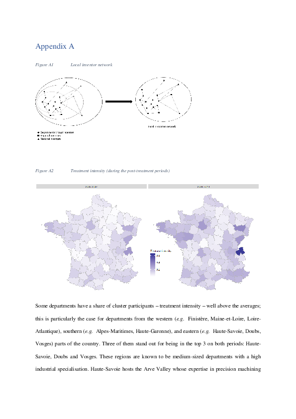
Appendix A Figure A1 Local inventor network Figure A2 Treatment intensity (during the post-treatment periods) Some departments have a share of cluster participants – treatment intensity – well above the averages; this is particularly the case for departments from the western (e.g. Finistère, Maine-et-Loire, LoireAtlantique), southern (e.g. Alpes-Maritimes, Haute-Garonne), and eastern (e.g. Haute-Savoie, Doubs, Vosges) parts of the country. Three of them stand out for being in the top 3 on both periods: HauteSavoie, Doubs and Vosges. These regions are known to be medium-sized departments with a high industrial specialisation. Haute-Savoie hosts the Arve Valley whose expertise in precision machining has been developed from the region’s clock and watch making industry during the 19th century. The Arve Valley’s expertise is nowadays recognised throughout the world and precision machining in the Haute-Savoie department accounts for 30% of its GDP and 70% of total French sales for this sector. Regarding the Doubs department, since the 17th century it has been shaped by the watchmaking industry thanks to an internationally recognised know-how in the various stages of watch manufacture. Following the watchmaking crisis of the 1970s and 1980s, the department has gradually diversified its industrial base towards microtechnology and is now considered as one of the leading French territories in the field of microengineering. Finally, the Vosges, often referred to as the “Wood Valley” is the leading French department for the volume of wood production (over 1 million m³ per year). The wood industry has always occupied an important place in the local economy and the department is home to a complete wood-based industry, ranging from timber harvesting to primary and secondary manufacturing (construction and high-end furnishings). To date, the department hosts more than 1,000 establishments and 13,000 jobs in the wood industry as well as the only public engineering school in France specialising in technologies related to wood and natural fibres. Most of the other departments having a high treatment intensity are also characterised by a certain level of industrial specialisation, although in smaller extent than those already mentioned. This descriptive analysis confirms the close link between the treatment intensity and territorial specialisation. Figure A3 Spatial distribution of the outcome variables (averaged over the pre-treatment periods) Figure 3 shows the spatial distribution of the outcome variables, averaged over the pre-treatment periods. Regarding the network small worldliness of local inventor networks during the pre-policy periods, it turns out the most small-world networks (i.e. networks characterised by high clustering coefficient and low average path length) were mainly those of the west coast, such as Morbihan, Loire-Atlantique, Vendée and Charente-Maritime. Although there were other departments also depicting a strong small world nature (e.g. Ardennes, Bouches-du-Rhône), it is worth noting that some innovative territories such as Rhône were characterized by a limited small world nature, compared to other departments. This can result from a high level of clustering which was very often coupled with a high average path length. Based on the first two maps on top, we can also notice that many of the dense local inventor network had a limited small world nature, suggesting that dense network may not necessarily be characterised by strong small worldliness. By increasing network small worldliness, the cluster policy would make local inventor networks more efficient. Furthermore, during the pre-policy periods, many local inventor networks were not resilient to the extent that as hierarchical structure was very often coupled with assortativity. Therefore, even though there were core actors able to coordinate local inventor networks, those actors tended to collaborate mainly with each other. There were, of course, some exceptions, mainly among small to medium-sized departments such as Lot, Finistère, Marne, Orne, and Vienne. It is worth noting the growing and innovative department that is Rhône – which is known for having a high concentration of chemical industries – was one of these exceptions. Figure A4 Spatial distribution of the outcome variables (averaged over the post-treatment periods) Table A1. Pre- and Post-treatment comparisons (Paired Student’s t-test) Dependent variables Number of observations Pre-treatment mean (Periods 1 & 2) Post-treatment mean (Periods 3 & 4) Density 94 0,016 0,014 Small World Quotient (SWQ) 94 6,625 6,228* Hierarchy 94 0,629 0,595*** Assortativity 94 0,887 0,83*** Note: Statistical significance: *p< 0.10, **p< 0.05, ***p< 0.01 Based on Table 4 and Figures 3 and 4, the comparison of the network features before and after the policy exhibits small variations on average. Network density faces a small but insignificant decline. The regions ranking remains very similar over the pre- and post-treatment periods. The small world quotient is also characterised by a small and insignificant reduction. However, converse to density, this mean stability hides important changes at the regional level. Some regions with weak small-worldliness properties before the policy turn to belong to the first or second quartile during the post-treatment period (Mayenne, Dordogne, Lot and Garonne, Hautes-Alpes). Conversely, other regions reduce their small world properties after the policy (Aisne, Ardennes, Yonne, Nièvre, Creuse, Corrèze, Landes, Aude). As most of these regions do not host clusters and record very few cluster participants and low treatment intensity (see Figure 2), these dynamics can however hardly result from the implementation of the French cluster policy. More minor changes are observed in highly treated regions, like in Paris area where a slight increase in small-worldliness is observed. The role played by more general trends or other shocks requires to be identified in order to determine to what extent the policy could have driven these transformations. More significant trends in network properties are observed from the last two dependent variables, namely hierarchy and assortativity. Both indicators exhibit smaller values after the policy implementation pointing to a reduction in the core-periphery structure of the network. Although some of the regions facing important changes are similar to the one above mentioned, others record a high treatment intensity (Alpes Maritimes, Morbihan, Vendée), pointing to potential relationships between policy participation and network dynamics. Beyond these descriptive statistics our econometric strategy thus aims at identifying the specific role played by the cluster policy. Table A2. Definition of the variables Variables Definitions Data sources nb_nodes (log) Number of inventors in the regional network INPI patent data gdp (log) Regional gross domestic product INSEE (National Institute of Statistics and Economic Studies) dird (log) Regional internal Research and Development expenditure sub_region (log) Total amount of regional subsidies received by local R&D firms sub_nat (log) Total amount of national subsidies received by local R&D firms sub_cee (log) Total amount of European subsidies received by local R&D firms RTA_Chemistry Regional level of specialisation in Chemistry RTA_Electrical_engineering Regional level of specialisation in Electrical engineering RTA_Instruments Regional level of specialisation in Instruments RTA_Mechanical_engineering Regional level of specialisation in Mechanical engineering Tc (continuous treatment variable) Number of regional participants to the cluster policy over the total number of R&D firms in the region DGE (General Division of Enterprises) and R&D survey from the French research Ministry Td (dichotomous treatment variable) Dummy taking value 1 if the region records more than 25% of cluster participants in at least one cluster DGE (General Division of Enterprises) Density Ratio of the number of edges in the regional network to the number of possible edges in this network INPI patent data SWQ (log) Regional Small World quotient (regional clustering coefficient ratio / regional path length ratio) INPI patent data Hierarchy Regional slope of the degree distribution Assortativity Regional slope of the degree correlation R&D survey from the French research Ministry R&D survey from the French research Ministry R&D survey from the French research Ministry R&D survey from the French research Ministry INPI patent data INPI patent data INPI patent data INPI patent data INPI patent data INPI patent data Table A3. Descriptive statistics of the variables Statistic N Mean St. Dev. Min Pctl(25) Pctl(75) Max nb_nodes (log) 376 5.780 1.262 1.609 4.903 6.553 8.817 gdp (log) 376 16.351 0.879 14.234 15.758 16.879 19.028 dird (log) 376 11.194 1.715 5.599 10.066 12.401 15.144 sub_region (log) 376 2.318 5.311 -6.908 0.704 5.937 10.085 sub_nat (log) 376 7.824 2.394 -6.908 6.485 9.254 13.456 sub_cee (log) 376 3.924 4.958 -6.908 3.268 7.09 10.265 RTA_Chemistry 376 0.849 0.375 0.000 0.592 1.073 1.995 RTA_Electrical_engineering 376 0.792 0.497 0.000 0.472 0.993 3.091 RTA_Instruments 376 0.861 0.353 0.000 0.621 1.084 2.379 RTA_Mechanical_engineering 376 1.136 0.354 0.438 0.883 1.331 2.556 Tc (on post-policy periods) 188 0.117 0.079 0.008 0.064 0.149 0.647 Density 376 0.015 0.022 0.0005 0.004 0.018 0.2 SWQ (log) 376 6.426 1.938 0.000 5.266 7.087 11.237 Hierarchy 376 0.612 0.104 0.28 0.551 0.651 1.117 Assortativity 376 0.858 0.107 0.493 0.79 0.94 1.000 Table A4. Operationalisation of outcome variables (to be continued) Variables Density Measurement The density of the (undirected) network is the ratio of the number of edges and the number of possible edges. It is calculated as follows: 𝐷= Where 𝑚 is the number of edges and 𝑛 is the number of nodes in the network. SWQ 2∙𝑚 𝑛 ∙ (𝑛 − 1) We proxy the level of network small worldliness using the widely adopted small world quotient (SWQ) which is defined as: 𝑆𝑊𝑄 = 𝐶𝐶𝑟𝑎𝑡𝑖𝑜 𝑃𝐿𝑟𝑎𝑡𝑖𝑜 The clustering coefficient (CC) ratio (𝐶𝐶𝑟𝑎𝑡𝑖𝑜 ) compares the actual clustering coefficient with the CC that can be expected in a random network of the same size and density. The formulas for calculating the clustering coefficient are as follows: 𝐶𝐶 = 𝑛𝑢𝑚𝑏𝑒𝑟 𝑜𝑓 𝑡𝑟𝑖𝑎𝑛𝑔𝑙𝑒𝑠 𝑤𝑖𝑡ℎ 𝑎𝑡 𝑙𝑒𝑎𝑠𝑡 𝑡ℎ𝑟𝑒𝑒 𝑙𝑒𝑔𝑠 𝑛𝑢𝑚𝑏𝑒𝑟 𝑜𝑓 𝑡𝑟𝑖𝑎𝑛𝑔𝑙𝑒𝑠 𝑤𝑖𝑡ℎ 𝑎𝑡 𝑙𝑒𝑎𝑠𝑡 𝑡𝑤𝑜 𝑙𝑒𝑔𝑠 𝐶𝐶𝑟𝑎𝑡𝑖𝑜 = 𝐶𝐶𝑎𝑐𝑡𝑢𝑎𝑙 𝐶𝐶𝑟𝑎𝑛𝑑𝑜𝑚 The path length (PL) ratio (𝑃𝐿𝑟𝑎𝑡𝑖𝑜 ) compares the actual average path length with the average path length that can be expected in a random network of the same size and density. The formulas for calculating the path length ratio are as follows: 𝑃𝐿 = 1 ∑ 𝑑(𝑣𝑖 , 𝑣𝑗 ) 𝑛 ∙ (𝑛 − 1) 𝑖,𝑗 where 𝑑(𝑣𝑖 , 𝑣𝑗 ) is the geodesic distance between nodes 𝑖 and 𝑗; 𝑛 is the number of nodes in the network. 𝑃𝐿𝑟𝑎𝑡𝑖𝑜 = 𝑃𝐿𝑎𝑐𝑡𝑢𝑎𝑙 𝑃𝐿𝑟𝑎𝑛𝑑𝑜𝑚 Variables Hierarchy Measurement The level of network hierarchy is reflected by the slope of the degree distribution, i.e., the relation between nodes degree and their rank position. We sort nodes by degrees from the largest to the smallest and transform them in log-log scale. Following Crespo et al. (2014; 2016), we consider that all nodes have at least one relation to avoid non-existing logs for isolate nodes. 𝑘ℎ = 𝐶(𝑘ℎ∗ )𝑎 log(𝑘ℎ ) = log(𝐶) + 𝛿log (𝑘ℎ∗ ) Where 𝑘ℎ denotes the degree 𝑘 of node ℎ, 𝑘ℎ∗ denotes the rank of node h in the distribution, 𝐶 is a constant, and a is the slope of relation. By construction, 𝛿 will take 0 or negative values. To simplify interpretation, we transform it in absolute terms. If 𝛿 has a high value, in absolute terms, the network will display a high level of hierarchy. Assortativity The level of assortativity or disassortativity of networks is reflected by the degree correlation, i.e., the slope of the relation between nodes’ degree and the mean degree of their local neighbourhood. For each node (inventor) ℎ, we calculate the mean degree of its neighbourhood 𝑉ℎ . A node 𝑖 is in the neighbourhood of node ℎ when both of them have, at least, one co-invention together, i.e., they have a relation. If 𝑘ℎ is the degree of node 𝑘, the mean degree of node ℎ is calculated as follows: ̅̅̅ 𝑘ℎ = 1 ∑ 𝑘𝑖 𝑘ℎ 𝑖∈𝑉ℎ And the relationship between nodes’ degree and the mean degree of their neighbourhood is estimated as follows: ̅̅̅ 𝑘 ℎ = 𝛼 + 𝛽𝑘ℎ Where 𝛼 is a constant and 𝛽 is the degree correlation. By construction, 𝛽 is enclosed between -1 and 1. If 𝛽 is positive and gets closer to 1, then the network is highly assortative, meaning that highly connected nodes tend to interact with highly connected nodes, and poorly connected nodes with poorly connected nodes. However, if 𝛽 is negative and gets closer to -1, the network is disassortative, meaning that highly connected nodes tend to interact with poorly connected nodes and vice versa. Table A5. Correlation matrix of the variables nb_nodes (log) gdp (log) dird (log) sub_regi on (log) sub_nat (log) sub_cee (log) RTA_Ch emistry RTA_El ectrical_ engineer ing RTA_In strument s RTA_M echanica l_engine ering Tc (on postpolicy periods) Density SWQ Hierarch y nb_nodes (log) 1.000 gdp (log) 0.922 1.000 dird (log) 0.918 0.855 1.000 sub_region (log) 0.398 0.407 0.441 1.000 sub_nat (log) 0.749 0.739 0.813 0.471 1.000 sub_cee (log) 0.686 0.647 0.753 0.364 0.676 1.000 RTA_Chemistry RTA_Electrical_e ngineering 0.344 0.367 0.329 0.119 0.249 0.226 1.000 0.297 0.239 0.319 0.180 0.301 0.255 -0.143 1.000 RTA_Instruments RTA_Mechanical _engineering Tc (on post-policy periods) 0.273 0.273 0.251 0.199 0.282 0.142 0.144 0.179 1.000 -0.309 -0.336 -0.299 -0.299 -0.339 -0.202 -0.381 -0.523 -0.598 1.000 0.291 0.198 0.300 0.200 0.237 0.220 -0.021 0.185 0.165 -0.152 1.000 Density -0.704 -0.646 -0.693 -0.296 -0.597 -0.555 -0.242 -0.185 -0.051 0.152 -0.247 1.000 SWQ (log) 0.199 0.255 0.207 0.019 0.215 0.163 0.107 0.051 0.048 -0.066 0.047 -0.296 1.000 Hierarchy -0.207 -0.191 -0.282 -0.204 -0.279 -0.191 -0.136 -0.172 -0.044 0.162 0.016 0.253 -0.224 1.000 Assortativity -0.544 -0.405 -0.545 -0.317 -0.426 -0.347 -0.124 -0.270 -0.104 0.126 -0.023 0.309 0.015 0.460 Assortati vity 1.000 Table A6. Coefficient estimates of spatial panel models (continuous treatment variable) SWQ 0.140* 0.106 0.126* 0.139* 0.142** 0.107 0.811 0.007 0.147* 0.020* -0.957 0.020 -0.001 – – – – -0.017 6.167* 0.024 0.379*** nb_nodes (log) -0.009*** -0.392 0.078*** -0.080 -0.010 -0.47 0.077*** -0.095 gdp (log) -0.039*** 7.522*** -0.362*** -0.056 -0.029** 6.215** -0.316*** -0.111 dird (log) 0.002 0.081 -0.027 0.001 0.003 -0.002 -0.026 -0.006 sub_region (log) 0.000 -0.002 -0.001 -0.002 0.000 0.005 -0.001 -0.001 sub_nat (log) -0.003 0.144 -0.009** -0.001 -0.003 0.141 -0.009** -0.001 sub_cee (log) 0.000 -0.068* 0.003* 0.002 0.000 -0.062* 0.003* 0.002* 0.008*** 0.797 -0.002 0.008 0.007*** 0.871* -0.005 0.013 0.004 -0.588 0.028 -0.041** 0.003 -0.447 0.023 -0.034* RTA_Instruments 0.007*** 0.598 0.026 -0.012 0.007*** 0.605 0.024 -0.013 RTA_Mechanical_engineering 0.012*** -0.956 0.054* -0.021 0.011*** -0.889 0.048 -0.020 W*Tc RTA_Chemistry RTA_Electrical_engineering Note: Statistical significance: *p< 0.10, **p< 0.05, ***p< 0.01 0.116 0.152** 0.017 Model 5 Hierarchy Density Tc SWQ Model 4 Hierarchy Assortativity Coefficients ρ Density Assortativity Table A7. Coefficient estimates of spatial DiD models (dichotomous treatment variable) Density SWQ – – constant 0.087 Td_25% Model 3 Hierarchy Model 4 (in DiD design) SWQ Hierarchy Assortativity Density – – -0.047 0.086 -0.069 0.192** -0.085 0.062 -0.069 0.124 7.587 0.421 1.106*** 0.031 -6.331 1.329 0.573** 0.052 -8.735 1.207 0.451* 0.004 0.074 -0.021 0.019 -0.001 0.148 0.007 0.010 -0.001 0.173 0.009 0.017 – – – – – – – – -0.007 1.073* 0.054 0.104 nb_nodes (log) 0.001 -0.006 0.007 0.0002 -0.013 -0.111 0.043** -0.046*** -0.013 -0.142 0.042** -0.05*** gdp (log) -0.004 -0.093 0.009 -0.014 0.001 0.730* -0.032 0.050*** 0.001 0.744* -0.032 0.047** dird (log) -0.002 -0.001 -0.001 -0.007 -0.002 0.188 -0.026* -0.029** -0.002 0.222 -0.024* -0.025** sub_region (log) -0.001 0.026 -0.000 0.001 -0.001** -0.036 0.008*** 0.006** -0.001** -0.044 0.008*** 0.006** sub_nat (log) 0.003* 0.028 0.002 0.005 0.004*** -0.135 -0.008 -0.006 0.003*** -0.113 -0.007 -0.004 sub_cee (log) 0.000 0.028 -0.002 -0.001 -0.001** 0.062 0.000 0.003* -0.001** 0.051 0.000 0.002 RTA_Chemistry 0.006 -0.112 -0.004 0.022 0.011*** -0.076 -0.031 -0.010 0.011*** -0.022 -0.028 -0.004 RTA_Electrical_engineering -0.003 -0.391 -0.002 -0.011 0.008** 0.02 -0.047** -0.048** 0.007** 0.128 -0.042* -0.039** RTA_Instruments -0.003 -0.248 0.01 0.028 0.011*** -0.242 0.017 0.008 0.011*** -0.12 0.023 0.021 RTA_Mechanical_engineering -0.01 0.154 0.005 -0.005 0.012* 0.000 -0.027 -0.042 0.010 0.365 -0.009 -0.009 D -0.006 0.356 0.008 -0.022 0.000 -0.481 0.019 0.047* 0.001 -0.504 0.018 0.046* Coefficients ρ W*Td_25% Note: Statistical significance: *p< 0.10, **p< 0.05, ***p< 0.01 Density Model 5 (in DiD design) SWQ Hierarchy Assortativity Assortativity Table A8. Alternative specification of the dichotomous dependent variable (10% threshold) As a sensitivity analysis regarding the dichotomous specification of the treatment variable, we consider as treated units all NUTS3 regions hosting at least 10% of a cluster’s participants. Density SWQ – – constant 0.077 Td_10% Model 3 Hierarchy Model 4 (in DiD design) SWQ Hierarchy Assortativity Density – – -0.044 0.080 -0.058 0.214*** -0.037 0.069 -0.056 0.210** 7.347 0.384 1.242*** 0.03 -7.532 1.299 0.526* 0.027 -8.312 1.286 0.449* 0.0001 -0.072 -0.028 0.058** -0.003 -0.129 -0.023 0.025 -0.003 -0.12 -0.023 0.027 – – – – – – – – 0.001 0.472 0.007 0.050** nb_nodes (log) 0.0004 -0.051 0.012 -0.004 -0.013 -0.069 0.041** -0.052*** -0.013 -0.095 0.041** -0.055*** gdp (log) -0.003 -0.064 0.011 -0.023 0.002 0.806* -0.029 0.052*** 0.002 0.809* -0.029 0.052*** dird (log) -0.002 0.027 -0.003 -0.005 -0.002 0.152 -0.023* -0.026** -0.002 0.147 -0.023* -0.026** sub_region (log) -0.001 0.026 -0.000 0.000 -0.001** -0.032 0.008*** 0.005** -0.001** -0.026 0.008*** 0.006** sub_nat (log) 0.003* 0.021 0.003 0.005 0.004*** -0.126 -0.009 -0.007 0.004*** -0.126 -0.009 -0.007 sub_cee (log) 0.000 0.031 -0.002 -0.001 -0.001** 0.060 0.000 0.004* -0.001** 0.063 0.000 0.004** RTA_Chemistry 0.006 -0.199 0.004 0.011 0.011*** 0.055 -0.037 -0.021 0.011*** 0.081 -0.037 -0.018 RTA_Electrical_engineering -0.003 -0.41 -0.003 -0.009 0.008** 0.042 -0.05** -0.046** 0.008** 0.07 -0.05** -0.043** RTA_Instruments -0.003 -0.241 0.013 0.022 0.011*** -0.22 0.017 0.008 0.011*** -0.188 0.018 0.012 RTA_Mechanical_engineering -0.011 0.063 0.009 -0.005 0.011* 0.041 -0.037 -0.047 0.012* 0.198 -0.034 -0.031 D -0.003 0.498 -0.004 -0.016 0.003 -0.544 0.053* 0.026 0.003 -0.542 0.053* 0.026 Coefficients ρ W*Td_10% Note: Statistical significance: *p< 0.10, **p< 0.05, ***p< 0.01 Density Model 5 (in DiD design) SWQ Hierarchy Assortativity Assortativity Table A9. Spatial DiD models (dichotomous treatment variable) Density Direct effects Td_25% W*Td_25% nb_nodes (log) gdp (log) dird (log) sub_region (log) sub_nat (log) sub_cee (log) RTA_Chemistry RTA_Electrical_engineering RTA_Instruments RTA_Mechanical_engineering DiD Indirect effects Td_25% W*Td_25% nb_nodes (log) gdp (log) dird (log) sub_region (log) sub_nat (log) sub_cee (log) RTA_Chemistry RTA_Electrical_engineering RTA_Instruments RTA_Mechanical_engineering DiD Total effects Td_25% W*Td_25% nb_nodes (log) gdp (log) dird (log) sub_region (log) sub_nat (log) sub_cee (log) RTA_Chemistry RTA_Electrical_engineering RTA_Instruments RTA_Mechanical_engineering DiD Model 4 (in DiD design) SWQ Hierarchy Assortativity Density Model 5 (in DiD design) SWQ Hierarchy Assortativity -0.001 – -0.013 0.001 -0.002 -0.001** 0.004 -0.001*** 0.011*** 0.008** 0.011*** 0.012* 0.000 0.148 – -0.111 0.731** 0.189 -0.036 -0.135 0.062 -0.076 0.02 -0.242 0.000 -0.482 0.007 – 0.043** -0.032 -0.026** 0.008*** -0.008 0.000 -0.031 -0.047** 0.017 -0.027 0.019 0.010 – -0.046*** 0.05*** -0.029** 0.006*** -0.006 0.003* -0.01 -0.048*** 0.009 -0.043 0.048* -0.001 -0.007 -0.013 0.001 -0.002 -0.001** 0.003 -0.001** 0.011*** 0.008** 0.011*** 0.010 0.001 0.173 1.074* -0.142 0.744 0.223 -0.044 -0.113 0.051 -0.022 0.128 -0.120 0.365 -0.504 0.009 0.054* 0.042** -0.032 -0.024* 0.008*** -0.007 0.000 -0.028 -0.042* 0.023 -0.009 0.018 0.017 0.105 -0.05*** 0.047*** -0.025** 0.006** -0.004 0.002 -0.004 -0.039** 0.021 -0.009 0.046* 0.000 – 0.001 0.000 0.000 0.000 0.000 0.000 -0.001 0.000 -0.001 -0.001 0.000 0.014 – -0.01 0.067 0.017 -0.003 -0.012 0.006 -0.007 0.002 -0.022 0.000 -0.044 0.000 – -0.003 0.002 0.002 -0.001 0.001 0.000 0.002 0.003 -0.001 0.002 -0.001 0.002 – -0.011 0.011 -0.007 0.001 -0.001 0.001 -0.002 -0.011 0.002 -0.010 0.011 0.000 0.001 0.001 0.000 0.000 0.000 0.000 0.000 -0.001 -0.001 -0.001 -0.001 0.000 0.011 0.07 -0.009 0.048 0.014 -0.003 -0.007 0.003 -0.001 0.008 -0.008 0.024 -0.033 -0.001 -0.003 -0.003 0.002 0.002 0.000 0.000 0.000 0.002 0.003 -0.002 0.001 -0.001 0.002 0.014 -0.007 0.007 -0.003 0.001 -0.001 0.000 -0.001 -0.005 0.003 -0.001 0.006 -0.001 – -0.013 0.001 -0.002 -0.001** 0.003*** -0.001** 0.011*** 0.008** 0.011** 0.011* 0.000 0.162 – -0.122 0.799** 0.206 -0.04 -0.148 0.068 -0.083 0.022 -0.264 0.000 -0.526 0.007 – 0.041** -0.03 -0.024** 0.008*** -0.008 0.000 -0.029 -0.044** 0.016 -0.025 0.018 0.012 – -0.057*** 0.062** -0.035** 0.008** -0.008 0.004* -0.013 -0.059** 0.010 -0.053 0.059* -0.001 -0.006 -0.012 0.001 -0.002 -0.001** 0.003 -0.001** 0.010*** 0.007* 0.010** 0.009 0.001 0.184 1.144* -0.151 0.793 0.237 -0.047 -0.121 0.055 -0.024 0.137 -0.127 0.388 -0.537 0.008 0.050* 0.039* -0.030 -0.022* 0.007** -0.007 0.000 -0.026 -0.039* 0.022 -0.008 0.017 0.020 0.119 -0.057*** 0.054** -0.029** 0.006** -0.005 0.003 -0.005 -0.045** 0.024 -0.010 0.052* Note: Statistical significance: *p< 0.10, **p< 0.05, ***p< 0.01