Academia.edu no longer supports Internet Explorer.
To browse Academia.edu and the wider internet faster and more securely, please take a few seconds to upgrade your browser.
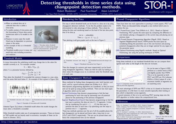
Detecting thresholds in time series data using changepoint detection methods
Detecting thresholds in time series data using changepoint detection methods
Detecting thresholds in time series data using changepoint detection methods
Detecting thresholds in time series data using changepoint detection methods
Detecting thresholds in time series data using changepoint detection methods
 Paul Fearnhead
Related Papers
2012 •
Time-series data often experiences abrupt changes in structure. If the time-series is to be modelled accurately then these changepoints must be taken into account. Many methods for detecting these changepoints, both heuristic and exact, have been developed and these are reviewed in this report. The report in particular looks at dynamic programming approaches and pruning methods which can be used to speed these methods up. The report concludes by discussing a few of the open questions which are still unresolved and ...
Journal of the American Statistical Association
Optimal Detection of Changepoints With a Linear Computational Cost2012 •
Journal of Computational and Graphical Statistics
Computationally Efficient Changepoint Detection for a Range of Penalties2017 •
2018 •
This thesis focuses upon the detection and prediction of changepoints in time series. In particular, we develop a range of methods, both parametric and non-parametric, to detect, predict, and forecast in the presence of changepoints. We consider a range of data applications. These include economic, environmental and telematics data sets. The first part of this thesis concentrates on forecasting. We propose two approaches to incorporate changepoints into the forecasting process. Each of these approaches are flexible. Additionally, we develop methodology to predict future changepoints in a time series. In particular, we can predict changepoints at both future time points, and changes near the end of the time series for which we do not yet have enough observations to detect. This also includes a new approach to pre-whitening time series that accounts for changes in the second order structure of the explanatory time series. The second part of this thesis is concerned with changepoint de...
Journal of Statistical Software
Generalized Functional Pruning Optimal Partitioning (GFPOP) for Constrained Changepoint Detection in Genomic Data2022 •
Journal of Computational and Graphical Statistics
Detecting Changes in Slope With an L0 Penalty2018 •
2020 •
Peak detection in genomic data involves segmenting counts of DNA sequence reads aligned to different locations of a chromosome. The goal is to detect peaks with higher counts, and filter out background noise with lower counts. Most existing algorithms for this problem are unsupervised heuristics tailored to patterns in specific data types. We propose a supervised framework for this problem, using optimal changepoint detection models with learned penalty functions. We propose the first dynamic programming algorithm that is guaranteed to compute the optimal solution to changepoint detection problems with constraints between adjacent segment mean parameters. Implementing this algorithm requires the choice of penalty parameter that determines the number of segments that are estimated. We show how the supervised learning ideas of Rigaill et al. (2013) can be used to choose this penalty. We compare the resulting implementation of our algorithm to several baselines in a benchmark of labele...
arXiv: Computation
A log-linear time algorithm for constrained changepoint detection2017 •
Changepoint detection is a central problem in time series and genomic data. For some applications, it is natural to impose constraints on the directions of changes. One example is ChIP-seq data, for which adding an up-down constraint improves peak detection accuracy, but makes the optimization problem more complicated. We show how a recently proposed functional pruning technique can be adapted to solve such constrained changepoint detection problems. This leads to a new algorithm which can solve problems with arbitrary affine constraints on adjacent segment means, and which has empirical time complexity that is log-linear in the amount of data. This algorithm achieves state-of-the-art accuracy in a benchmark of several genomic data sets, and is orders of magnitude faster than existing algorithms that have similar accuracy. Our implementation is available as the PeakSegPDPA function in the coseg R package, https://github.com/tdhock/coseg
Statistics and Computing
A computationally efficient nonparametric approach for changepoint detection2016 •
RELATED PAPERS
Journal of the American Statistical Association
Changepoint Detection in the Presence of Outliers2018 •
2021 •
Journal of the American Statistical Association
Detecting Abrupt Changes in the Presence of Local Fluctuations and Autocorrelated Noise2021 •
Environmental Challenges
Insights into the hydrogeological framework of the NW Himalayan Karewas (India)Journal of Computational and Graphical Statistics
Subset Multivariate Collective and Point Anomaly Detection2021 •
American Journal of Theoretical and Applied Statistics
The Power of the Pruned Exact Linear Time(PELT) Test in Multiple Changepoint Detection2015 •
Algorithms for Molecular Biology
Segmentor3IsBack: an R package for the fast and exact segmentation of Seq-data2014 •
Journal of the Royal Statistical Society: Series A (Statistics in Society)
Change point analysis of historical battle deathsJournal of Statistical Software
changepoint : An R Package for Changepoint Analysis2014 •
BMC Bioinformatics
MPAgenomics: an R package for multi-patient analysis of genomic markers2014 •
Pacific Symposium on Biocomputing. Pacific Symposium on Biocomputing
TrackSigFreq: subclonal reconstructions based on mutation signatures and allele frequencies2020 •
arXiv: Methodology
Scalable changepoint and anomaly detection in cross-correlated data with an application to condition monitoring2020 •
2022 •
2015 •
Journal of Probability and Statistics
Parametric Methodologies for Detecting Changes in Maximum Temperature of Tlaxco, Tlaxcala, México2019 •
Journal of the Royal Statistical Society: Series C (Applied Statistics)
A novel regularized approach for functional data clustering: an application to milking kinetics in dairy goatsCommunications for Statistical Applications and Methods
Real-time prediction for multi-wave COVID-19 outbreaksComputational Statistics & Data Analysis
Fast estimation of posterior probabilities in change-point analysis through a constrained hidden Markov model2013 •
Journal of Agricultural, Biological, and Environmental Statistics
Comparing Segmentation Methods for Genome Annotation Based on RNA-Seq Data2014 •
arXiv: Machine Learning
Lagged Exact Bayesian Online Changepoint Detection with Parameter Estimation2017 •
Computational Statistics & Data Analysis
A comparison of single and multiple changepoint techniques for time series data2022 •
Signal Processing
Fast estimation of the Integrated Completed Likelihood criterion for change-point detection problems with applications to Next-Generation Sequencing data2014 •
Statistical Methods in Medical Research
Periodic-type auto-regressive moving average modeling with covariates for time-series incidence data via changepoint detection2019 •
2018 •
Journal of Computational and Graphical Statistics
Simultaneous Credible Regions for Multiple Changepoint Locations2018 •
2018 •
Problems in oncology
Urokinase and Its Receptor in Cutaneous Melanoma Reproduced in Chronic Neurogenic Pain in Mice of Both Genders in Comparison2020 •
The Annals of Statistics
Consistent selection of the number of change-points via sample-splittingResearch Studies in Music Education
Soundtrap usage during COVID-19: A machine-learning approach to assess the effects of the pandemic on online music learningProceedings of the 26th IEEE International Symposium on Computer-Based Medical Systems
ACLAC: An approach for adaptive closed-loop anesthesia control2013 •
- Find new research papers in:
- Physics
- Chemistry
- Biology
- Health Sciences
- Ecology
- Earth Sciences
- Cognitive Science
- Mathematics
- Computer Science