This art icle was downloaded by: [ Pedro Garcia]
On: 30 Novem ber 2011, At : 15: 26
Publisher: Taylor & Francis
I nform a Lt d Regist ered in England and Wales Regist ered Num ber: 1072954 Regist ered
office: Mort im er House, 37- 41 Mort im er St reet , London W1T 3JH, UK
Applicable Analysis
Publicat ion det ails, including inst ruct ions f or aut hors and
subscript ion inf ormat ion:
ht t p: / / www. t andf online. com/ loi/ gapa20
Synchronization of non-identical
extended chaotic systems
A. Acost a
a
, P. García
b
& H. Leiva
c
a
Depart ament o de Mat emát ica Aplicada, Facult ad de Ingeniería,
Universidad Cent ral de Venezuela, Caracas, Venezuela
b
Laborat orio de Sist emas Complej os, Depart ament o de Física
Aplicada, Facult ad de Ingeniería, Universidad Cent ral de
Venezuela, Caracas, Venezuela
c
Escuela de Mat emát ica, Facult ad de Ciencias, Universidad de
Los Andes, Mérida, Venezuela
Available online: 30 Nov 2011
To cite this article: A. Acost a, P. García & H. Leiva (2011): Synchronizat ion of non-ident ical
ext ended chaot ic syst ems, Applicable Analysis, DOI: 10. 1080/ 00036811. 2011. 635654
To link to this article: ht t p: / / dx. doi. org/ 10. 1080/ 00036811. 2011. 635654
PLEASE SCROLL DOWN FOR ARTI CLE
Full t erm s and condit ions of use: ht t p: / / www.t andfonline.com / page/ t erm s- andcondit ions
This art icle m ay be used for research, t eaching, and privat e st udy purposes. Any
subst ant ial or syst em at ic reproduct ion, redist ribut ion, reselling, loan, sub- licensing,
syst em at ic supply, or dist ribut ion in any form t o anyone is expressly forbidden.
The publisher does not give any warrant y express or im plied or m ake any represent at ion
t hat t he cont ent s will be com plet e or accurat e or up t o dat e. The accuracy of any
inst ruct ions, form ulae, and drug doses should be independent ly verified wit h prim ary
sources. The publisher shall not be liable for any loss, act ions, claim s, proceedings,
dem and, or cost s or dam ages what soever or howsoever caused arising direct ly or
indirect ly in connect ion wit h or arising out of t he use of t his m at erial.
Applicable Analysis
2011, 1–12, iFirst
Synchronization of non-identical extended chaotic systems
A. Acostaa, P. Garcı́ab* and H. Leivac
a
Departamento de Matemática Aplicada, Facultad de Ingenierı´a, Universidad Central de
Venezuela, Caracas, Venezuela; bLaboratorio de Sistemas Complejos, Departamento de
Fı´sica Aplicada, Facultad de Ingenierı´a, Universidad Central de Venezuela, Caracas,
Venezuela; cEscuela de Matemática, Facultad de Ciencias, Universidad de Los Andes,
Me´rida, Venezuela
Downloaded by [Pedro Garcia] at 15:26 30 November 2011
Communicated by S. Leonardi
(Received 18 May 2011; final version received 24 October 2011)
In this article a technique to achieve synchronization in spatially extended
systems is introduced. The basic idea behind this method is to map a system
of partial differential equations (PDEs) into a high-dimensional space
where the representation of this PDE is an ordinary differential equation.
By using semi-group theory, we are able to find conditions that ensure the
synchronization of two systems of non-identical reaction–diffusion
equations with a master–slave coupling.
Keywords: chaos synchronization; reaction-diffusion equations; coupled
systems
AMS Subject Classifications: 70G60; 74H65; 35K57
1. Introduction
Synchronization in chaotic finite-dimensional systems is a subject that has been
having great attention since 1983 with the seminal article of Fujisaka and Yamada
[1]. However from 1990, with the work of Pecora and Carroll [2], the interest for the
phenomenon has increased enormously and different techniques, based on some well
establish theories (e.g. Lyapunov functions [3,4], exponential dichotomies theory [5],
are some examples) have been applied.
On the other hand, for spatially extended systems the synchronization is a very
complicated problem and several techniques, in order to achieve this, have been
implemented. Particularly, the scheme based on linear feedback control method has
been very useful for synchronizing identical [6–11] and non-identical [12–16]
infinite-dimensional chaotic systems.
In order to study synchronization for non-identical spatially extended chaotic
systems, we follow an approach based on semi-group theory. The idea behind our
scheme is very simple, we consider an infinite-dimensional system and represent it in
an abstract setting which corresponds to an ordinary differential equation in
*Corresponding author. Email: pedro@fisica.ciens.ucv.ve
ISSN 0003–6811 print/ISSN 1563–504X online
ß 2011 Taylor & Francis
http://dx.doi.org/10.1080/00036811.2011.635654
http://www.tandfonline.com
2
A. Acosta et al.
a Hilbert space. Specifically, we consider a system of two vector reaction–diffusion
equations linearly coupled using a master–slave scheme. Although, the setting is very
formal, we explicitly exhibit the relation involving the parameters in the problem,
and this allows us to estimate the intensity of the coupling as a function of the
difference between the initial condition and the control parameters of the systems.
2. Setting of the problem
We consider the system of two vector-coupled reaction–diffusion equations
ð1Þ ð2Þ
utð1Þ ¼ d1 uð1Þ
xx þ f1 ð, u , u Þ
Downloaded by [Pedro Garcia] at 15:26 30 November 2011
ð2Þ
ð1Þ ð2Þ
uð2Þ
t ¼ d2 uxx þ f2 ð, u , u Þ,
ð1Þ
vð1Þ , vð2Þ Þ þ ðuð1Þ vð1Þ Þ
vð1Þ
t ¼ d1 vxx þ f1 ð,
ð2Þ
vð1Þ , vð2Þ Þ þ ðuð2Þ vð2Þ Þ,
vð2Þ
t ¼ d2 vxx þ f2 ð,
ð1Þ
ð2Þ
with t > 0, 0 < x < l, homogeneous Dirichlet conditions: u(i)(0, t) ¼ v(i)(0, t) ¼ 0,
u(i)(l, t) ¼ v(i)(l, t) ¼ 0, i ¼ 1, 2 and where , which is the coupling intensity, is a real
positive number, di, i ¼ 1, 2, are positive constants and fi: Rm R R ! R, i ¼ 1, 2,
are continuous functions.
In a compact form, Equations (1) and (2), can be written as
ut ¼ Duxx þ Fð, uÞ
and
vÞ þ ðu vÞ,
vt ¼ Dvxx þ Fð,
ð3Þ
ð4Þ
where u ¼ (u(1), u(2))T, v ¼ (v(1), v(2))T, D is a diagonal matrix with elements D11 ¼ d1
and D22 ¼ d2 and F(, u) ¼ ( f1(, u), f2(, u))T. The boundary conditions are
expressed as u(0, t) ¼ v(0, t) ¼ 0, and u(l, t) ¼ v(l, t) ¼ 0. Notice that, without
considering the coupling term, the systems (3)–(4) differs only in the parameter .
The function F, because its components are continuous, is continuous. Also, we
assume the following hypothesis:
H1. Given a ball Br(0), with radius r and centre 0 in R2, there exists a constant
L ¼ L(r, ) > 0 such that
jFð, u1 Þ Fð, u2 Þj Lju1 u2 j
for all u1 , u2 2 Br ð0Þ:
H2. There exists K > 0, such that
uÞj Kj jjuj
jFð, uÞ Fð,
for all , 2 Rm , u 2 R2 :
In addition to the previous hypothesis it is important to remark that throughout
this work we assume and as constant vectors.
Next, we rewrite system (3)–(4) in terms of the difference u v by using a solution
of Equation (3) (master equation). Let u0(x, t) be a bounded solution of Equation (3)
that satisfies u0(0, t) ¼ u0(l, t) ¼ 0, and consider it as an input in Equation (4)
(slave equation).
Applicable Analysis
3
Now consider the transformation z ¼ u v, with u ¼ u0, i.e.
z ¼ u0 ðx, tÞ v:
ð5Þ
If v is a solution of the slave equation with input u0, then the transformation (5)
applied to this equation yields the following equation:
u0 zÞ
zt ¼ Dzxx z þ Fð, u0 Þ Fð,
ð6Þ
and z satisfies the boundary conditions
zð0, tÞ ¼ zðl, tÞ ¼ 0
t 4 0:
ð7Þ
Downloaded by [Pedro Garcia] at 15:26 30 November 2011
We will obtain synchronization through the study of the problem (6)–(7). It means
existence of solutions with v being arbitrarily close to u0 as t tends to þ1.
3. Abstract formulation of the problem
In this section, by choosing an appropriate space, we will set our problem as an
abstract ordinary differential equation.
Let X ¼ L2((0, l ), R2) and consider the linear unbounded operator
A: D(A) X ! X defined by
d2
A ¼ D 2 þ I ,
ð8Þ
dx
where I is the identity operator, and
DðAÞ ¼ H10 ðð0, l Þ, R2 Þ \ H2 ðð0, l Þ, R2 Þ:
H2((0, l), R2) being the Sobolev space W2, 2((0, l), R2) and H10 ðð0, l Þ, R2 Þ the closure of
the set C10 ðð0, l Þ, R2 Þ, the C2-functions with compact support, in the norm of
W2,2((0, l), R2).
The spectrum (A), of the operator A, consists of just eigenvalues n,i ¼
di(n/l)2 þ , n ¼ 1, 2, . . . , i ¼ 1, 2. We order the set of eigenvalues {n,i} according to
the sequence 0 < 1 < 2 < ; where 1 ¼ min{d1, d2}(/l)2 þ . For each n the
corresponding eigenspace has dimension n, where n 2 {1, 2}.
In this framework there exists a complete orthonormal set fg1
n¼1 of eigenvectors
of A, where each element in this set has the form either ð2l Þ1=2 ðsinðjl xÞ, 0ÞT or
ð2l Þ1=2 ð0, sinðjl xÞÞT with j 2 {1, 2, . . .}. Therefore for all 2 D(A) we have the
representation
A ¼
1
X
h, n in ,
n¼1
where h, i is the inner product in X. Also, A generates an analytic semigroup
{eAt} given by
eAt ¼
1
X
n¼1
en t h, n in :
4
A. Acosta et al.
In order to study the non-linear part of the abstract differential equation
corresponding to the problem (3)–(4), we need to consider the fractional power space
X , 0 , associated with A. X is defined as X ¼ D(A ) and, because X is a Hilbert
space, it has the structure of Hilbert space. Moreover,
1
X
n h, n in ,
A ¼
n¼1
and the norm induced by the inner product on X is given by
1
X
kk2 :¼
n jh, n ij2 :
n¼1
ð9Þ
Downloaded by [Pedro Garcia] at 15:26 30 November 2011
The next proposition contains estimates relating the semi-group {eAt} with the
norms kk and kk.
PROPOSITION 1
For each 2 X we have the following estimates:
keAt k e1 t kk ,
where M ¼ ð e Þ
Proof
=2
keAt k Mt
and
t 0:
=2 21 t
e
kk,
t 4 0,
> 0.
From the above notation, for 2 X we have
*
+2
1
1
X
X
keAt k2 ¼
ej t , j j , i
i
j¼1
i¼1
¼
1
X
i¼1
2
i ei t h, i i
e21 t
1
X
i¼1
i jh, i ij2
¼ e21 t kk2 :
Therefore,
keAt k e1 t kk :
The second inequality follows from the fact that, for > 0, the sequence of functions
defined by fn ðtÞ ¼ ðn tÞ en t , n ¼ 1, 2, . . . ; t 0, satisfies the estimate fn(t) ( /e)
uniformly in n and t. In fact,
keAt k2 ¼
1
X
i¼1
¼ t
i e2i t jh, i ij2
1
X
i¼1
ei t fi ðtÞjh, i ij2
t e1 t
2
M t e
1
X
i¼1
1 t
fi ðtÞjh, i ij2
k k 2 :
5
Applicable Analysis
Therefore,
keAt k Mt
=2 21 t
e
kk:
g
From Theorem 1.6.1 in [17] we obtain, for 1/2 < < 1, that there exists
~ 2 Cðð0, l Þ, R2 Þ such that ¼
~ almost everywhere and the operators i1:
X ! C((0, l), R2) and i2: X ! X defined by
~
i1 ðÞ ¼ ,
i2 ðÞ ¼
are continuous. Hence for the inclusions
Downloaded by [Pedro Garcia] at 15:26 30 November 2011
X Cðð0, l Þ, R2 Þ
and X X
there are constants C > 1 and R > 0, such that
sup jðxÞj Ckk
x2ð0,l Þ
and kk Rkk ,
2X
ð10Þ
Now, we associate to the system (3)–(4) the following ordinary differential equation
with initial condition on the space X:
_ þ A ¼ Fe ð, ,
, tÞ
ðt0 Þ ¼ 0 ,
t t0 4 0,
ð11Þ
where Fe: Rm Rm X [0, þ1) ! X is given by
, tÞðxÞ :¼ Fð, u0 ðx, tÞÞ Fð,
u0 ðx, tÞ ðxÞÞ:
Fe ð, ,
ð12Þ
From now on, we will suppose that 1/2 < < 1.
Let us assume that u0(, t) 2 X , t > 0, and it is uniformly bounded, i.e. there exists
an N > 0 such that
ku0 ð, tÞk N
for all t 4 0:
ð13Þ
The following lemma contains important estimates concerning to Fe, and shows that
Equation (11) is well posed in X .
LEMMA 1 (a) Given a ball with radius and centre zero in X , there exists a constant
L 4 0 such that for 1 , 2 2 B ð0Þ
1 2 k
1 , tÞ Fe ð, ,
2 , tÞk Lk
kFe ð, ,
ð14Þ
(b) There exists a constant K 4 0 such that
j,
0, tÞk Kj
kFe ð, ,
for all , 2 Rm , t > 0.
Proof
4 0 such that
(a) For H1, given r > 0 there exist a constant L ¼ Lðr, Þ
u2 Þj Lju1 u2 j
u1 Þ Fð,
jFð,
for all u1 , u2 2 B ð0Þ:
ð15Þ
6
A. Acosta et al.
Choosing r ¼ C(N þ ), with C as in (10) and N as in (13), we get
1 , tÞðxÞ Fe ð, ,
2 , tÞðxÞj
D ¼ jFe ð, ,
u0 ðx, tÞ 2 ðxÞÞ Fð,
u0 ðx, tÞ 1 ðxÞÞj
¼ jFð,
LðCðN þ Þ, Þj
1 ðxÞ 2 ðxÞj:
Therefore, if 1 , 2 2 B ð0Þ, then
1 , tÞ Fe ð, ,
2 , tÞk LðCðN þ Þ, Þk
kFe ð, ,
1 2 k:
Finally, the second estimate in (10) implies that
1 2 k
1 , tÞ Fe ð, ,
2 , tÞk Lk
kFe ð, ,
Downloaded by [Pedro Garcia] at 15:26 30 November 2011
with L ¼ RLðCðN þ Þ, Þ:
(b) For H2,
0, tÞðxÞj ¼ jFð, u0 ðx, tÞÞ Fð,
u0 ðx, tÞÞj Kj jju
0 ðx, tÞj:
jFe ð, ,
Now, by using (10) and (13), respectively, we get
0, tÞðxÞj Kj jCku
jFe ð, ,
0 ð, tÞk Kj jCN:
Therefore,
Z
l
0
and
0, tÞj2 dx lK2 C2 N2 j j
2
jFe ð, ,
j,
0, tÞk Kj
kFe ð, ,
where K ¼ KCNl1=2 .
g
From Lemma 1 of this article and Lemma 3.3.2 of [17], for all T > t0 we have the
following: a continuous function (): (t0, T ) ! X is solution of the integral
equation
Zt
ðsÞ, sÞds, t 2 ðt0 , TÞ,
eAðtsÞ Fe ð, ,
ð16Þ
ðtÞ ¼ eAðtt0 Þ 0 þ
t0
if and only if () is a solution of (11).
4. Existence of bounded solutions
Consider Cb([0, 1), X ), the space of the bounded and continuous functions defined
on the interval [0, 1) and taking values in X . Cb([0, 1), X ) is a Banach space with
the supremum norm
kkb :¼ supfkðtÞk : t 0g,
2 Cb ð½0, 1Þ, X Þ:
A ball of radius > 0 and centre zero in this space is given by
Bb ¼ f 2 Cb ð½0, 1Þ, X Þ : kkb g:
Now, we are ready to establish the main result of this article.
7
Applicable Analysis
K the constants in the Lemma 1. If the
THEOREM 1 Let be a positive number and L,
following estimate holds:
1 =2
þ Kj
j
M L
1
,
ð17Þ
4 ð1 =2Þ
2
where M ¼ ( /e) /2 and is the well-known gamma function, then Equation (11) admits
one and only one bounded solution 2 Bb .
Proof Let S be the set of all functions 2 Bb . With the norm that has been defined
previously, S is a complete metric space. Next, inspired by (17), we define for 2 S
Zt
ðsÞ, sÞds:
eAðtsÞ Fe ð, ,
ð18Þ
TðÞðtÞ ¼
Downloaded by [Pedro Garcia] at 15:26 30 November 2011
0
We have that T() is continuous. Now, the estimates giving in Lemma 1
imply that
ðsÞ,sÞ Fe ð, ,
0,sÞ þ Fe ð, ,
0, sÞ L kkb þ K j j:
ðsÞ, sÞ ¼ Fe ð, ,
Fe ð, ,
Therefore, using the second estimate in Proposition 1 and a change of variables,
its follows that
Zt
ðsÞ, sÞ ds
eAðtsÞ Fe ð, ,
TðÞðtÞ
0
Zt
1
Mðt sÞ2 e 2 ðtsÞ L kkb þ K j j ds
0
¼ M L kkb þ K j j
Z
1
2t
Z0
1
M L kkb þ K j j
es s2 ds
es s2 ds
0
2 12
¼ M Lkkb þ Kj j
1
1
2
12
þ K j j 2
M L
1 :
1
2
Hence, kT()(t)k and T(S ) S.
Now, we are going to establish that T is a contraction on S. For all 1, 2, t > 0,
we have
D :¼ kTð2 ÞðtÞ Tð1 ÞðtÞk
Zt
2 ðsÞ, sÞ Fe ð, ,
1 ðsÞ, sÞÞk ds
keAðtsÞ ðFe ð, ,
0
Zt
1
2 ðsÞ, sÞ Fe ð, ,
1 ðsÞ, sÞk ds
Mðt sÞ2 e 2 ðtsÞ kFe ð, ,
0
Zt
1
ML ðt sÞ2 e 2 ðtsÞ k2 ðsÞ 1 ðsÞkds
0
12
2
ML
1
1
2
k2 1 kb :
8
A. Acosta et al.
2 Þ12 ð1 Þ 5 1 and this implies that T is a
Now, from (17) we have MLð
1
2
contraction. The above discussion allows us to conclude that T has a unique fixed
~ 2 S,
point
Zt
~
~
ðsÞ,
ðtÞ ¼
eAðtsÞ Fe ð, ,
sÞds:
0
~ is the solution defined on (0, 1), of the initial value problem with
Moreover,
g
t0 ¼ 0 and 0 ¼ 0, given for Equation (11).
Downloaded by [Pedro Garcia] at 15:26 30 November 2011
When the initial condition in Equation (11) is not zero, a similar result could be
obtained.
K the constants in the Lemma 1. If the
THEOREM 2 Let be a positive number and L,
following estimate holds
1 =2
þ k0 kb þ Kj
j
M L
1
,
ð19Þ
4 2 ð1 =2Þ
2
where M ¼ ( /e) /2, then the Equation (19) admits one and only one bounded solution
~ 0 2 Bb .
2 Bb . Moreover, for all t > 0, ðtÞ
Notice that, if ¼ and (0 ¼ 0, we have two identical systems with the same
initial condition, in this case the system starts synchronizing and remains in that
state. If 6¼ and 0 6¼ 0, then for each > 0 there exists a critical value c such that
the systems synchronize for each > c. Also, it is important to mention that in the
case of identical systems, inequalities (17) and (19) imply local synchronization, i.e. if
the solutions for t ¼ 0 are sufficiently close, they converge to each other as t goes to
infinity. However, the inclusion of the parameter makes our result a bit more
general than local synchronization.
5. Numerical results
In order to show the performance of our technique, we use the Gray–Scott cubic
autocatalysis model [18]
@u1
@ 2 u1
¼ d1 2 u1 u22 þ að1 u1 Þ
@t
@x
@u2
@ 2 u2
¼ d2 2 þ u1 u22 ða þ bÞu2 :
@t
@x
This reaction–diffusion system correspond to two irreversible chemical reactions and
exhibits mixed mode spatiotemporal chaos. Here, b, the dimensionless rate constant
of the second reaction and a the dimensionless feed rate and di, i ¼ 1, 2, are the
diffusion coefficients. As in reference [7], the constants associated with the system are
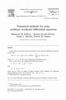
chosen as: a ¼ 0.028, b ¼ 0.053, d2 ¼ 105, d1 ¼ 2d2 and l ¼ 2.5.
Figure 1 shows the evolution of the component u1 of the Gray–Scott system.
It displays, with the set of parameters given, the spatiotemporal chaotic behaviour
associated to the system.
9
Applicable Analysis
u1
10 000
8000
t
6000
4000
Downloaded by [Pedro Garcia] at 15:26 30 November 2011
2000
0
0.0
0.5
1.0
1.5
2.0
2.5
x
Figure 1. Contour plot of component u1, of the Gray–Scott system.
In our case, we have two of this reaction–diffusion systems coupled by mean of a
master–slave scheme:
@u1
@ 2 u1
¼ d1 2 u1 u22 þ að1 u1 Þ
@t
@x
@u2
@ 2 u2
¼ d2 2 þ u1 u22 ða þ bÞu2
@t
@x
@v1
@ 2 v1
v1 Þ þ ðu1 v1 Þ
¼ d1 2 v1 v22 þ að1
@t
@x
@v2
@ 2 v2
2 þ ðu2 v2 Þ:
¼ d2 2 þ v1 v22 ða þ bÞv
@t
@x
The vector field F(a, b, u1, u2) is given by ðu1 u22 þ að1 u1 Þ, u1 u22 ða þ bÞu2 Þ, and
satisfies the condition H1 with L ¼ 2(4r2 þ a þ b), and satisfies a ¼ a condition H2
with K ¼ 1.
On the other hand, the constants C and R appearing in (10) can be chosen as
C¼
1
1
=2 1=2
l
,
R¼
1
1 =2
:
Now, we realize a numerical implementation to illustrate the second theorem.
We use the previous values for the constants a and b, a ¼ 0.028, b ¼ 0:049, ¼ 0.75
and , chosen according to (17) as 0.24 and 5 103, respectively. Also, according
10
A. Acosta et al.
0.1
e(t)
10–4
10–7
10–10
10–13
0
200
400
600
800
1000
Downloaded by [Pedro Garcia] at 15:26 30 November 2011
t
Figure 2. Semi-logarithmic plot of the global error of synchronization versus the time. The
solid line shows the before-mentioned error for different initial conditions and non-identical
systems with given parameters and the dotted line shows the same results in the case of
identical systems.
to the expression for L and K given in the Lemma 1, we obtain
!
pffiffiffi
1
3
2
N
2
ðN þ Þ þ a þ b , K ¼
L ¼
:
2
l
12
1
1
The initial conditions are given by
x ,
l
u2 ðx, 0Þ ¼ sin x ,
l
u1 ðx, 0Þ ¼ sin
2
2
v1 ðx, 0Þ ¼ ðe10ðxl=3Þ þ e1000ðx2l=3Þ Þ sin
x ,
l
2
1
v2 ðx, 0Þ ¼ e10ðxl=2Þ sin x :
2
l
Figure 2 shows a semi-logarithmic plot of the global error of synchronization,
which is defined by
( Z
)1=2
2
1 lX
eðtÞ ¼
ð20Þ
ðui ðx, tÞ vi ðx, tÞÞ2 dx
l 0 i¼1
versus time t. Here we show that the error (20) behaves in such a way that it cannot
be greater than the value assign to . As can be seen, the synchronization error
becomes very small in an exponential way. The solid line shows the above-mentioned
error for different initial conditions and non-identical systems with given parameters
and the dotted line shows same results in the case of identical systems.
6. Concluding remarks
As a final comment, we want remark that in contrast with the works in [6–15], in this
work the synchronization is achieved from an analytic result instead of numeric
Applicable Analysis
11
search of the conditions for synchronization. Although the scheme is illustrated with
a coupled reaction–diffusion equations, the methodology is quite general and
seems to be useful in studying synchronization of other types of extended chaotic
systems.
Acknowledgements
This work was partially supported by Consejo de Desarrollo Cientı́fico y Humanı́stico de la
Universidad Central de Venezuela and CDCHT-ULA, Project C1667-09-05-AA.
We also thank the second referee as we believe that their suggestions have improved the
presentation and had suggested interesting lines of future research.
Downloaded by [Pedro Garcia] at 15:26 30 November 2011
References
[1] H. Fujisaka and T. Yamada, Stability theory of synchronized motion in coupled-oscillator
systems, Prog. Theor. Phys. 69 (1983), pp. 32–47.
[2] L.M. Pecora and T.L. Carroll, Synchronization in chaotic systems, Phys. Rev. Lett. 64
(1990), pp. 821–824.
[3] C.W. Wu and L.O. Chua, A unified framework for synchronization and control of
dynamical systems, Int. J. Bifurcation Chaos 4(4) (1994), pp. 979–998.
[4] H.M. Rodrigues, Abstract methods for synchronization and applications, Appl. Anal.
62(3–4) (1996), pp. 263–296.
[5] A. Acosta and P. Garcı́a, Synchronization of non-identical chaotic systems: An exponential
dichotomies approach, J. Phys. A: Math. Gen. 34 (2001), pp. 9143–9151.
[6] L. Kokarev, Z. Tasev, T. Stojanovski, and U. Parlitz, Synchronizing spatiotemporal chaos,
Chaos. 7(4) (1997), pp. 635–643.
[7] L. Kocarev, Z. Tasev, and U. Parlitz, Synchronization of spatiotemporal chaos of partial
differential equations, Phys. Rev. Lett. 79(1) (1997), pp. 51–54.
[8] C. Beta and A.S. Mikhailov, Controlling spatiotemporal chaos in oscillatory
reaction–diffussion systems by time-delay autosynchronization, Physica D. 199(1–2)
(2004), pp. 173–184.
[9] A. Amengual, E. Hernandez-Garcı́a, R. Montangne, and M. San Miguel, Synchronization
of spatiotemporal chaos. The regime of coupled spatiotemporal intermittency, Phys. Rev.
Lett. 78 (1997), pp. 4379–4382.
[10] J. Bragard, S. Boccaletti, and H. Mancini, Asymmetric coupling effects in the
synchronization of spatially extended chaotic systems, Phys. Rev. Lett. 91(6) (2003),
p. 064103-1-064103-4.
[11] L. Junge and U. Parlitz, Phys. Synchronization and control of couple complex
Ginzburg-Landau equations using local coupling, Phys. Rev. E. 61(4) (2000),
pp. 3736–3742.
[12] A.E. Hramov, A.A. Koronovskii, and P. Popov, Generalized synchronization in coupled
Ginzburg–Landau equations and mechanisms of its arising, Phys. Rev. E. 72 (2005),
p. 037201-1-037201-4.
[13] C.T. Zhou, Synchronization in nonidentical complex Ginzburg–Landau equations, Chaos.
16(013124) (2006), pp. 013124–013131.
[14] S. Boccaletti, J. Bragard, F.T. Arecchi, and H. Mancini, Synchronization in nonidentical
extended systems, Phys. Rev. Lett. 83(3) (1999), pp. 536–339.
[15] J. Bragard, F. Arecchi, and S. Boccaletti, Characterization of synchronized spatiotemporal
states in coupled nonidentical complex Ginzburg–Landau equations, Int. J. Bifurcation
Chaos. 10(10) (2000), pp. 2381–2389.
12
A. Acosta et al.
Downloaded by [Pedro Garcia] at 15:26 30 November 2011
[16] P. Garcı́a, A. Acosta, and H. Leiva, Synchronization conditions for master–slave reaction
diffusion systems, Europhys. Lett. 88(6) (2009), pp. 60006p1–60006p4.
[17] D. Henry, Geometric Theory of Semilinear Parabolic Equations, Springer-Verlag,
New York, 1981.
[18] P. Gray and S.K. Scott, Sustained oscillations and other exotic patterns in isothermal
reactions, J. Phys. Chem. 89(25) (1985), pp. 22–32.
Academia.edu no longer supports Internet Explorer.
To browse Academia.edu and the wider internet faster and more securely, please take a few seconds to upgrade your browser.
Related Papers
Download

International Journal of Control, 2011
Download

Communications in Partial Differential Equations, 2003
Download

Cognitive Neurodynamics, 2014
Download

Communications in Nonlinear Science and Numerical Simulation, 2014
Download


European Journal of Control, 2010
Download

International Journal of Systems Science, 2007
Download

Journal of Differential Equations, 2003
Download

Applied Mathematics and Computation, 2012
Download

Journal of vibration and acoustics
Download


International Journal of Solids and Structures, 2010
Download

Applied Mathematics and Computation, 2006
Download

Applied Mathematics and Computation, 2005
Download