COMPARISON OF NEAR-FIELD EVENTS AND THEIR FAR-FIELD
ACOUSTIC SIGNATURES IN EXPERIMENTAL AND NUMERICAL
HIGH SPEED JETS
Pinqing Kan
Syracuse University
pkan@syr.edu
Jacques Lewalle
Syracuse University
jlewalle@syr.edu
Guillaume Daviller
Institut Pprime, Université de Poitiers and Cerfacs, Toulouse
daviller@cerfacs.fr
ABSTRACT
Two different approaches are applied to near-field (NF)
velocity field and far-field (FF) pressure signals to gain better understanding of the flow structures that contribute to
high speed jet noise. We use laboratory data from a 10kHz
TRPIV experiment data of Mach 0.6 jet and numerical data
from an 80kHz LES database at Mach 0.9 jet. From the
NF, over 20 representative diagnostics are extracted as time
traces, of which about half give high correlation with the
far-field. Utilizing cross-correlation and wavelet analysis,
we locate the frequency band where information is transferred from NF to FF. Furthermore we identify excerpts in
time and frequency domain that act as major correlation
contributors. The lists of events based on FF only (acoustic footprints) and on NF-FF correlations are compared and
show good similarity, which validates both techniques. Finally, the lists of events are separated into categories based
on their properties, including magnitude, frequency, and
time of occurrence.
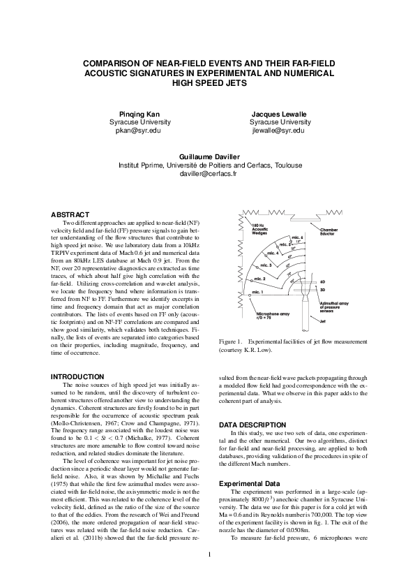
Figure 1. Experimental facilities of jet flow measurement
(courtesy K.R. Low).
INTRODUCTION
sulted from the near-field wave packets propagating through
a modeled flow field had good correspondence with the experimental data. What we observe in this paper adds to the
coherent part of analysis.
The noise sources of high speed jet was initially assumed to be random, until the discovery of turbulent coherent structures offered another view to understanding the
dynamics. Coherent structures are firstly found to be in part
responsible for the occurrence of acoustic spectrum peak
(Mollo-Christensen, 1967; Crow and Champagne, 1971).
The frequency range associated with the loudest noise was
found to be 0.1 < St < 0.7 (Michalke, 1977). Coherent
structures are more amenable to flow control toward noise
reduction, and related studies dominate the literature.
The level of coherence was important for jet noise production since a periodic shear layer would not generate farfield noise. Also, it was shown by Michalke and Fuchs
(1975) that while the first few azimuthal modes were associated with far-field noise, the axisymmetric mode is not the
most efficient. This was related to the coherence level of the
velocity field, defined as the ratio of the size of the source
to that of the eddies. From the research of Wei and Freund
(2006), the more ordered propagation of near-field structures was related with the far-field noise reduction. Cavalieri et al. (2011b) showed that the far-field pressure re-
DATA DESCRIPTION
In this study, we use two sets of data, one experimental and the other numerical. Our two algorithms, distinct
for far-field and near-field processing, are applied to both
databases, providing validation of the procedures in spite of
the different Mach numbers.
Experimental Data
The experiment was performed in a large-scale (approximately 8000 f t 3 ) anechoic chamber in Syracuse University. The data we use for this paper is for a cold jet with
Ma = 0.6 and its Reynolds number is 700,000. The top view
of the experiment facility is shown in fig. 1. The exit of the
nozzle has the diameter of 0.0508m.
To measure far-field pressure, 6 microphones were
1
�Speed distribution, frame 1, Test 31
0.8
0.7
0.6
0.6
0.4
0.5
0.2
0
0.4
−0.2
0.3
−0.4
0.2
−0.6
0.1
−0.8
−1
4
4.2
4.4
4.6
4.8
5
5.2
5.4
5.6
5.8
0
Figure 3. Local instantaneous Mach number (black box is
for the region of window averaging).
Figure 2. Instantaneous flow visualization of LES data.
that relate near-field and far-field are recorded as ‘NF
events’. Another algorithm (Lewalle et al., 2012) uses
cross-correlation and wavelet analysis as well, however this
method focuses on the events that are shared by three farfield microphones and uses no near-field information. The
list of ‘FF events’ thus generated can be interpreted as footprints of near-field sources.
placed in the same horizontal plane with the jet center line.
Their distance from the center of the nozzle is 75 diameters, and they were located in 15o increments from the jet
center. The pressure signals were collected at 40.96 kHz
and low-pass filtered at 20.48 kHz. There were 8192 samples for each record. For the algorithm in this paper, we use
pressure signal at 15o microphone.
The near-field 2D velocity field was captured by a 10
kHz TR-PIV simultaneously (Low et al, 2013). 2 cameras
with 576 × 576 pixel resolutions sampled at 20kHz. A
Neodym-Yag laser output at 10 kHz in the same horizontal plane of jet centerline and was recorded in 8623 snapshots. A trigger signal was created to ensure the near-field
and far-field records were aligned simultaneously. These
tests (noted as test 31, 32 and 33) of measurements covered
approximately 4 ≤ x/D ≤ 8 in the streamwise location and
−1 ≤ y/D ≤ 1 in the spanwise. Each test took about 1.5D
in the spanwise and had the same transverse locations. The
end of the potential core was measured in Test 33, which is
counted as the key region of jet noise production.
Near-field and Far-field Cross-Correlation
For each NF velocity snapshot, we perform a window
averaging (black box in fig. 3) and extract a series of dimensionless statistics. These quantities from successive frames
are then recorded respectively in time traces. The statistics
include:
√
• the average speed < u2 + v2 >;
• the absolute value of transverse (radial) component of
velocity <| v |>;
• the rms value of | v |;
• the rms value of v;
• the absolute value of Reynolds stress <| uv− < u ><
v >|>
• the absolute value large-scale vorticity <| ω |>;
• the rms value of ω;
• the absolute value of 2-D divergence (trace of rate-ofstrain) <| ∂x u + ∂y v |>;
• the rms value of ∂x u + ∂y v = sxx + syy ;
• the absolute value of the determinant of 2-D rate-ofstrain <| sxx syy − s2xy |>;
• the rms value of sxx syy − s2xy .
• the Q criterion < (||Ω||2 − ||S||2 )/2 >=<
−∂ j ui ∂i u j /2 >;
• the absolute value of Q <| ||Ω||2 − ||S||2 | /2 >;
LES Data
The LES data simulated an isothermal jet with Ma =
0.9 and has the Reynolds number being 400,000. The sampling rate is 80kHz. The numerical algorithm and computation schemes can be found in Daviller (2010), and the details will not be shown here. Fig. 2 is one example of the
instantaneous flow field, where the coherent structures are
represented by the isosurfaces of Q criterion. The pressure
at radial r/D = 6 and axial x/D = 15 are sampled as farfield signals (D = 0.02 m). For the near-field, the database
was filtered to reduce the size by a factor of 33 . This is applicable at present since we are looking for the relationship
between near-field coherent structures and jet noise, which
doesn’t require the full resolution. Another simplification is
the usage of 2D plane instead of full 3D field. The diagnostics listed before are then replicated for the 2D sections.
Looking for the relationship between near-field flow structures and far-field noise, we filtered and down sampled the
far-field pressure to match the PIV acquisition rate, and applied cross-correlation and wavelet analysis to the diagnostics and pressure signals.
The cross-correlation reaches the maximum at the lag
that corresponds to acoustic propagation time (fig. 4). The
time of sound propagation is estimated by dividing the
Cartesian distance by ambient speed of sound, resulting in
a typical 10.5 ms expected lag between NF and FF. As the
distance decreases (from top row to bottom row), it can
be observed in fig. 4 the corresponding reduction of lags.
EXTRACTION OF EVENTS RELATED TO
NOISE PRODUCTION
Two independent algorithms will be presented in this
section. The first makes use of both near-field velocity
field and far-field pressure, after applying cross-correlation,
wavelet analysis and pattern recognition scheme, the events
2
�Ma−ave
x/D = 5
0.1
|v|
10.5ms,−0.062818
|div(u)|
10.4ms,0.11004
|rey|
10.4ms,0.11687
0.03
|Q|
10.5ms,0.10022
9.5 ms
9.7 ms
9.7 ms
10.0 ms
10.2 ms
10.4 ms
10.6 ms
10.8 ms
10.4ms,0.10107
0
0.02
−0.1
x/D = 5.5
0.1
10.3ms,−0.10639
10.4ms,0.11922
10.3ms,0.11817
10.4ms,0.10655
10.3ms,0.088257
0.01
0
−0.1
x/D = 6
0.1
10.2ms,−0.11119
10.2ms,0.10685
10.2ms,0.1324
10.2ms,0.10111
10.2ms,0.10551
10.1ms,−0.11264
10.1ms,0.10152
10ms,0.14134
10.1ms,0.10006
10ms,0.11972
0
0
−0.1
x/D = 6.5
0.1
−0.01
0
−0.02
−0.1
x/D = 7
0.1
9.9ms,−0.10931
10.1ms,0.10597
10ms,0.13015
10ms,0.097952
10ms,0.099037
−0.03
0.1
0
0.2
0.3
0.4
0.5
St
−0.1
−3 0
5
10 13
−3 0
lag(ms)
5
10 13
lag(ms)
−3 0
5
10 13
lag(ms)
−3 0
5
10 13
−3 0
lag(ms)
5
10 13
lag(ms)
Figure 5. Variation of cross-correlation of 2D divergence
and FF signals v.s. frequency (PIV data).
Figure 4. Cross-correlation of NF diagnostics and FF signals in the time domain (PIV data).
The largest value of peak cross-correlation appears roughly
around x/D = 6.5, which is near the end of potential core.
All the diagnostics show the pattern described above, and
this can be interpreted as the occurrence of yet-unknown
events influencing all these quantities in conjunction with
the noise production observed from the far-field.
These cross-correlations are resolved in frequency.
Taking the real part of the Morlet wavelet transform provides the narrow-band frequency resolution of the crosscorrelations. The formula below defines the transformed
coefficient of near-field signals in time-frequency domain.
NFM (t, ω) =
Z
NF(t + t ′ )ψM (ωt ′ )dt ′ .
(1)
Similarly the transformation of far-field pressure FFM (t, ω)
can be obtained. Then we can calculate the crosscorrelation in time-frequency domain by correlating at each
frequency level:
ρ(τ, ω) =
Z
NFM (t, ω) FFM (t + τ, ω) dt.
Figure 6. Contributions to cross-correlation in TFL domain; red is positive, blue negative.
(2)
we use a pattern recognition scheme to extract the contributions of correlation in time and frequency domain. Morlet
wavelet is again applied to the near- and far-field signals and
the real part of the transformation coefficients are correlated
without averaging in frequency levels (fig. 6). The strong
red or blue patches represent the main correlation contributors where the signals are locally in phase or half a period
out of phase. The oscillations, e.g., at 15 < t < 17ms, can
be viewed as short wave packets in the time domain. The
first two frames show the phase shift of half a period as we
change the lags. Different diagnostics share a lot of common patterns (e.g. last frame).
Viewing the highly correlated red or blue patches as
noise-related events, we tested for false positives resulting
from the chance occurrence of such patches. Indeed, any
unstructured signal, when band-pass filtered, will contain
local oscillations. The correlation contour plots of white
Gaussian noise and of incorrectly-lagged (i.e. presumably
independent) signals look very similar to fig. 6. However,
the patches are as likely to be positive as negative at every
frequency level and they tend to cancel out when averaged;
the incomplete cancellation for our finite record length gives
residual correlations of the order of 3 to 5%, well below the
Two different normalizations are compared during this process. One is to normalize the filtered signals to unit variance and then correlate them. The resulted filtered correlation level reaches 30% to 40%. This method factors out
the energy information and makes the low-frequency event
stand out (below Strouhal 0.1). The other correlates the signals without normalization (fig. 5). The frequency range of
around Strouhal 0.2 becomes dominant, which is also that
of peak of energy spectrum. Focusing on the events that
offer more obvious physical interpretation for the present,
we are using the second normalization for the remaining
content. Different diagnostics again generate very similar
figures. Some difference exists in the sign of the peak correlation, which is caused by the in-phase or out-of-phase state
of the two compared signals. LES dataset gives very similar
patterns, with a shift towards higher frequency, which may
be caused by the higher Mach number.
Pattern Recognition of Individual Wave
Packets Moving from the statistical to the event level,
3
�St = 0.13761 Test 32 Xcor = 0.70192
2.5
Matched Events of all the diagnostics (%) =0.59524
0.016
2
Excerpts in Common
Unmatched
0.014
0.012
Morlet(p15)
1.5
1
0.5
0.01
0.008
0.006
0.004
0
0.002
0
−0.5
0.1
0.2
0.3
0.4
0.5
Strouhal
−3
−1
12
x 10
9
11
−1.5
10
Near−field
Far−field
−2
126
127
128
129
130
131
132
133
134
135
136
Magnitude
Time (ms)
St = 0.73275 Station 5.5 Xcor = −0.70946
2.5
7
8
6
7
5
6
5
2
1.5
8
9
4
4
3
3
2
2
1
1
0.1
0.2
0.3
0.4
0.5
Strouhal
0.5
0
−0.5
Figure 8. a. Distribution matched and unmatched events;
b. Property histogram of matched events.
−1
−1.5
−2
Near−field
Far−field
−2.5
8.05
8.1
8.15
8.2
8.25
8.3
8.35
8.4
8.45
8.5
Time (ms)
2.5
15o
30o
2
Figure 7. Matched events between near- and far-field (1st
frame for PIV and the other for LES data).
45o
45o alt.
Magnitude (arb. units)
1.5
10 to 20% level observed for the actual signals and the 25 to
35% level calculated with frequency resolution. While the
list of events obtained below will unavoidably contain some
false positives, the large majority of them cannot be due to
chance.
The local extrema of these instantaneous contributions
are collected over a range of lags oscillating approximately
1 period from that of peak cross-correlation. We extracted
the envelopes of the packets of oscillations as in Fig. 6.
Around the local peak value, we extracted a few periods and
calculated the excerpts’ cross-correlation between NF and
FF. The event is added to the list if the excerpt correlation
coefficient exceeds 0.6, and if the far-field magnitude is at
least twice the mean value. This ensures that the recorded
events are strong enough to be physically important. Fig.
7 shows two examples of the resulting excerpts, one from
PIV and the other from LES data.
In order to get some statistical level description of the
NF events, we collect the events recognized by all the diagnostics and keep those that are common to at least two of
them. About 250 out of 450 excerpts (about 60%) are kept
in this final list and they will be referred to as NF events
in this paper. Their distribution and property histogram is
shown in fig. 8. In the scattering plot, the x-positions of
the markers are shifted randomly from the original (within
20%) to alleviate the overlap. The magnitude vs. frequency
distribution resembles that of energy spectrum. The lower
frame shows the 2D histogram of number of events at different frequency and magnitude levels. The darkest spot,
representing the majority of the events are clustered around
Strouhal 0.2.
1
0.5
0
−0.5
−1
−1.5
−2
−2.5
20
21
22
23
24
25
26
27
28
Dimensionless time
Figure 9. Matched events at 15o , 30o , 45o microphones.
herence and are used to identify some of the loudest events.
Detailed algorithm description can be found in Lewalle et
al. (2012). Since 15o pressure has the most dominant coherent noise of the three, we make a list of local maxima
of its Morlet coefficients. These are the loudest events captured by this microphone. Then we keep three periods of
the Mexican hat coefficients centering at each of these loud
events. These short signals are then correlated with their
corresponding parts from the other two microphones. This
provides the lags between microphones for the events. If the
peak value of 15 − 30o cross-correlation is above 0.75, and
that of 15 − 45o exceeds 0.35, with its corresponding largest
lag not bigger than 35 time steps, we keep this as one FF
event (one example shown in fig. 9). We verified that the
list of FF events is not affected by the down-sampling to
10kHz.
COMPARISON OF NF EVENTS AND FF
EVENTS
Three levels of comparison of the FF and NF approaches are possible: statistical (using the entire length
of the available records), local (on an event-by-event basis), and collective (comparing the populations of events,
which amounts to conditional statistics). We will address
firstly the statistical and collective level and then perform
the event-by-event comparison.
Far-field Pressure Signatures of Individual
Noise Sources
The far-field acoustic signals contain the distorted signature of individual coherent near-field sources. The 15o ,
30o and 45o far-field microphones are within the cone of co-
4
�Figure 10. Distribution of peak cross-correlation contributions between Q (pressure source term) and far-field pressure.
Figure 12. Distribution of peak cross-correlation contributions between Ma and far-field pressure.
concur about the location of the sources of noise.
The statistical picture differentiates between diagnostics. Velocity-derivative diagnostics tend to agree with the
Q results shown above, with some additional activity at
8 < x/D < 10 which is tentatively interpreted as the turbulent aftermath of the noise production. However, velocitybased diagnostics paint a different picture. For example,
the local Mach number (dimensionless speed) is correlated
to far-field pressure mostly inside the potential core itself,
as seen in Fig. 12. The physical interpretation of this correlation is the subject of on-going work.
Green for large amplitude
1
0.8
0.6
0.4
y/D
0.2
0
−0.2
−0.4
−0.6
−0.8
−1
2
3
4
5
x/D
6
7
8
Comparison of Lists of Events and Some
Statistics
Figure 11. Location of sources obtained from the far-field
cross-correlation algorithm (LES data) and triangulation to
the near-field.
From the two independent algorithms described above,
we get two lists of events. Their excerpts, illustrated in fig.
9 for FF and fig. 7 for NF, are observed as short wave packets, which appear consistent with Cavalieri et al (2011a).
Distribution in Space/Frequency
• ‘FF events’ that are captured by 3 far-field microphones. These events are energetic and cluster near
the acoustic peak. They oscillate for 3 to 5 periods,
making a form of wave packets, even though the identification algorithm uses Mexican hat wavelet and does
not presuppose an oscillatory pattern. The list consists
of about 260 events.
• ‘NF events’ that are common to near-field kinematics
and far-field acoustics (15o microphone only). These
events are the connection between near-field and farfield but are not necessarily the loudest ones. This list
has about 150 events.
The statistical results are resolved according to streamwise and transverse location and according to frequency.
For a given diagnostic, we can plot the contributions to
cross-correlation with the far-field, as a percentage of the
largest value for this diagnostic. The most active regions are
mapped out as iso-surfaces of constant relative contribution
to the cross-correlation, in the (x-y-St) coordinates. The result for Q is shown in fig. 10, for the LES data. Iso-surfaces
for levels 50, 65 and 80% of maximum are superposed
and the color scale is from cyan to magenta for weaker to
stronger levels. In addition to being a topological index, Q
is also proportional to the source term in the incompressible pressure equation ∇2 p = − Q
ρ . Thus large correlation
of Q with the far-field pressure is indicative of actual production of far-field noise. We see that this active region is
located primarily in the shear layer, close to the centerline
near the tip of the potential core at 5.5 < x/D < 7.5, with
some residual activity farther downstream. The corresponding Strouhal number is in the vicinity of 0.3, matching the
peak of the far-field acoustic spectrum.
This statistical result agrees closely with the estimates
of source location obtained by triangulation from the FF
events, as shown in fig. 11. The algorithm for triangulation is based on the small differences in detection times
at 4 far field (numerical) microphones, which corresponds
to differences in distance between source and microphone.
The error bars cover the source locations that give similar
integer values of the lags at the available sampling rate of
80 kHz. We conclude that the FF events and NF correlations
To find the matches between these two lists of events,
we construct the following criteria: the time of occurrence
of two events are within one period
√ of each other, the frequencies are within a factor of 2 of each other, and their
magnitudes of filtered far-field pressure coefficient are less
than 25% apart on their respective scales. The last criteria is to make sure the very loud event is not too weak in
the other. With these being set, nearly 60% are found in
common. The same algorithm is tested by replacing the farfield signal by White Gaussian noise or incorrectly lagged
signals. This yields only about 10% in common. Therefore
it may be concluded that these two independent algorithms
identify many of the same events. This is also verification
of both of the algorithms.
The distribution and histograms of the matched and unmatched events can be found in fig. 13. The majority of the
matched events have frequency of about Strouhal 0.2 to 0.3
5
�Events in common:0.52 (%NF);0.53937 (%FF)
also surprising that about a dozen diagnostics show corre-
0.02
Common NF Events
Unmatched NF events
Common FF Events
Unmatched FF Events
0.018
0.016
8
0.8
Morlet(p15)
0.014
7
0.012
0.01
1. ave−Ma
2. |v|
3. |rey|
4. |div(u)|
5. |det(s)|
6. |vort|
7. |Q|
8. Q
0.7
6
0.6
5
0.5
0.008
0.006
0.004
4
0.002
0.4
0.3
3
0
0.1
0.2
0.3
0.4
0.5
0.2
Strouhal
2
−3
12
x 10
NF excerpts − matched
12
10
0
10
6
8
6
Magnitude
Magnitude
1
8
8
4
4
1
6
8
6
0.2
0.3 0.4 0.5
0.1
Strouhal
−3
x 10
0.2
0.3 0.4 0.5
Strouhal
Residue − NF excerpts
5
6
7
8
Residue − FF sources
−3
12
8
x 10
8
10
10
6
Magnitude
Magnitude
4
Figure 14. Percentage of matched events of 2-diagnostic
combinations.
2
0.1
6
3
4
2
2
8
2
4
2
12
0.1
FF events − matched
−3
x 10
4
4
8
6
6
4
lation to the far-field and their similarities and differences
will be investigated. We will also make use of the near-field
pressure information in future research.
This work was supported in part by a AFOSR grant,
Spectral Energies, a Syracuse University Graduate Fellowship and by an SU Research Growth Award of Mechanical Department. We are indebted to the members of the
Glauser group at SU for the data acquisition and processing and many discussions, particularly with Mark Glauser,
Kerwin Low, Patrick Shea and Zach Berger; and at Pprime
with Bernd Noack, Peter Jordan, Joel Delville and JeanPaul Bonnet. Several SU undergraduate students, G. Freedland, A. Tenney and V. Holcomb, participated in verification
of some of the algorithms.
4
2
2
2
2
0.1
0.2
Strouhal
0.3 0.4 0.5
0.1
0.2
0.3 0.4 0.5
Strouhal
Figure 13. Distribution and property histograms of
matched and unmatched events.
and show some difference in magnitude that is allowed by
the flexibility of matching algorithm. The unmatched events
are either too high or too low in frequency as NF events and
have very low magnitude as FF events.
DISCUSSION
REFERENCE
The connection between near-field kinematics and farfield acoustics of high speed jets has been observed in both
statistical and event level. Allowing for chance matches, the
interpretation of events as source-related is supported by the
large correlation coefficients. The large portion of similarity
between the results of two independent algorithms, which is
also high above the chance level, is another verification of
the relationship between extracted events to noise sources.
The FF events that are common to three far-field microphones signals display pattern of wave packets. For the
NF events, the wave packet shape may be an artifact of the
Morlet wavelet. But since this list shares about 50% of the
events with the former, it is reasonable to state that this
list of events also takes the wave packet form. Our algorithm generates very similar results for both experimental
and LES dataset, which helps to verify the reliability of the
scheme.
Although the diagnostics display a lot of common
features, some difference between velocity-related and
velocity-derivative-related diagnostics is emerging. Fig. 14
compares the diagnostics one by one. The RMS values are
not compared here since they are more like their original
values (70% in common on average). This is consistent
with our previous analysis (fig. 10). These two combinations seem to leads to two different populations of events
which capture different flow structures.
Some aspects that we would like to look further into
include: look at the PIV snapshots and try and identify the
mechanism of noise production; the portion of events that
are highly correlated between NF and FF but with unexpected low frequency needs to be understood further; it is
Cavalieri, A., Daviller, G., Comlte, P., Jordan, P., Tadmor, G. and Gervais, Y. 2011a, ”Using large eddy simulation to explore sound-source mechanisms in jets”, J. Sound
Vib., 330, 40984113.
Cavalieri, A. V. G., Jordan, P., Agarwal, A. and Gervais, Y., 2011b, ”Jittering wave-packet models for subsonic
jet noise”, J. Sound Vib. 330, 44744492.
Crow, S. C. and Champagne, F. H., 1971, ”Orderly
structure of jet turbulence”, J. Fluid Mech. 48, 547591.
Daviller, G., 2010, ”Numerical study of temperature
effects in round and coaxial jets”, PhD thesis, Ecole Nationale Sup erieure de M ecanique et dA erotechnique,
Poitiers, France.
Lewalle, J., Low, K. R. and Glauser, M. N., 2012,
”Properties of the far-field pressure signatures of individual
jet noise sources”, Int. J. Aeroacoustics, 11, 651 674.
Low, K. R., Berger, Z. P., Kostka, S., ElHadidi, B.,
Gogineni, S. and Glauser, M. N., 2013, ”A low-dimensional
approach to close-loop control of a mach 0.6 jet”, Exp. Fluids, 54, 117.
Michalke, A., 1977, ”On the effect of spatial source
coherence on the radiation of jet noise”, J. Sound Vib. 55,
377394.
Michalke, A. and Fuchs, H. V., 1975, ”On turbulence
and noise in an axisymmetric shear flow”, J. Fluid Mech.
70, 179205.
Mollo-Christensen, E., 1967, ”Jet noise and shear flow
instability seen from an experimenters viewpoint”, J. Appl.
Mech. 34, 17.
Wei, M. and Freund, J. B., 2006, ”A noise-controlled
free shear flow”, J. Fluid Mech. 546, 123152.
6
�
 Pinqing Kan
 Guillaume Daviller