MARINE ECOLOGY PROGRESS SERIES Mar Ecol Prog Ser Vol. 453: 227–240, 2012 doi: 10.3354/meps09636 Published May 7 OPEN ACCESS Global analysis of cetacean line-transect surveys: detecting trends in cetacean density R. Jewell1, 2,*, L. Thomas3, C. M. Harris2, 3, K. Kaschner4, R. Wiff5, P. S. Hammond2, N. J. Quick1, 6 1 SMRU Ltd., New Technology Centre, North Haugh, St. Andrews, Fife, KY16 9SR, Scotland Sea Mammal Research Unit, Scottish Oceans Institute, University of St. Andrews, St. Andrews, Fife, KY16 8LB, UK 3 Centre for Research into Ecological and Environmental Modelling, Buchanan Gardens, University of St. Andrews, St. Andrews, Fife, KY16 9LZ, UK 4 Evolutionary Biology and Ecology Lab, Institute of Zoology, Albert-Ludwigs-University, 79104 Freiburg, Germany 5 Instituto de Fomento Pesquero (IFOP), Blanco 839, Valparaíso, Chile 6 School of Biology, University of St. Andrews, St. Andrews, Fife, KY16 9TF, UK 2 ABSTRACT: Measuring the effect of anthropogenic change on cetacean populations is hampered by our lack of understanding about population status and a lack of power in the available data to detect trends in abundance. Often long-term data from repeated surveys are lacking, and alternative approaches to trend detection must be considered. We utilised an existing database of linetransect survey records to determine whether temporal trends could be detected when survey effort from around the world was combined. We extracted density estimates for 25 species and fitted generalised additive models (GAMs) to investigate whether taxonomic, spatial or methodological differences among systematic line-transect surveys affect estimates of density and whether we can identify temporal trends in the data once these factors are accounted for. The selected GAM consisted of 2 parts: an intercept term that was a complex interaction of taxonomic, spatial and methodological factors and a smooth temporal term with trends varying by family and ocean basin. We discuss the trends found and assess the suitability of published density estimates for detecting temporal trends using retrospective power analysis. In conclusion, increasing sample size through combining survey effort across a global scale does not necessarily result in sufficient power to detect trends because of the extent of variability across surveys, species and oceans. Instead, results from repeated dedicated surveys designed specifically for the species and geographical region of interest should be used to inform conservation and management. KEY WORDS: Marine mammal density · Population trends · Generalised additive modelling · Power analysis · Monitoring Resale or republication not permitted without written consent of the publisher INTRODUCTION Many anthropogenic activities in the marine environment, for example fisheries, human recreation, marine renewable energy development, mineral extraction, transport, and defence-related activities, are perceived to have a negative impact on marine fauna through direct competition for prey, bycatch, and as a result of both sound and chemical pollution. Many of these activities are likely to expand substantially over the next few decades and, for many species and geographical areas, we are poorly equipped to measure and quantify any consequences of these activities or to suggest marine planning approaches to mitigate potential effects. Demonstrating the existence of an effect or the impact of an activity on a species or *Email: rj67@st-andrews.ac.uk © Inter-Research 2012 · www.int-res.com 228 Mar Ecol Prog Ser 453: 227–240, 2012 population can be extremely complex, and often data are not available at appropriate spatial or temporal resolutions to make an assessment. We first have to determine whether it is possible to detect population level changes or trends, and it is this question that we aim to address in this paper. A recent review of the conservation status of the world’s mammals (Schipper et al. 2008) concluded not only that marine mammals are poorly known (with 38% of species data deficient), but that they face higher threat levels relative to terrestrial mammals: an estimated 36% of marine mammal species were considered threatened. A species’ conservation status is assigned based on quantitative criteria relating to its risk of extinction, including the population size and rate of decline as well as the extent of population fragmentation and geographic distribution. As a contributing factor to a species’ risk of extinction, the rate of change of a population is of high importance and a primary focus of much research. However trend detection can be complicated by a large range of factors. Many cetacean species are wideranging and not easily observed at sea, making abundance estimation problematic. To deal with these difficulties, researchers have developed a number of different methods for monitoring cetacean populations and analysing data, including, for example, photo-identification studies (e.g. Smith et al. 1999, Parra et al. 2006), land-based census methods (Zeh et al. 1991, Buckland & Breiwick 2002), linetransect surveys (e.g. SCANS surveys; Hammond et al. 2002, SCANS-II 2008) and acoustic monitoring (Barlow & Taylor 2005, Marques et al. 2009). Although all of these methods can provide a good means of monitoring populations, in order to detect trends in abundance (or density) we still need to address the problem of how robust and comparable data from multiple surveys are across years. Genuine variability among population estimates could be caused by taxonomic, spatial or temporal factors, whereas methodological factors could lead to biased estimates of density; both of these sources of variability may disguise the existence and directionality of underlying trends. If density estimates from multiple species are grouped together, because of sparse data for example, taxonomic differences will be evident as it is unlikely that all species within the same family are following the same population trend. Spatial differences will occur if survey areas vary among years, covering different parts of a species’ range or covering habitat of varying suitability. Temporal differences will occur if surveys of a population are conducted in different seasons or years, particularly if dealing with one of the many highly migratory cetacean species (e.g. Gilles et al. 2009). Methodological differences among population estimates may result if several survey or analysis techniques are used (e.g. estimates from Barlow 2003 and Barlow 2006). Within the same survey methodology, differences in how the data are analysed will result in variability in the resultant population estimates (Gómez de Segura et al. 2007). For example, accounting for animals missed from the transect line during line-transect surveys by estimating g(0) (the probability of animals being available for detection on the trackline) will likely result in higher estimates of density than if this bias is not accounted for (e.g. Laake et al. 1997, Heide-Jørgensen et al. 2008). Failing to consider this when looking at temporal trends in density could cause a bias in the trend estimate. For example, if g(0) was not accounted for in early surveys but was during later surveys a spurious increasing trend could result. Furthermore differences in the application of the same methodologies could be present among different research groups responsible for conducting the surveys. Variability in density estimates from different surveys, as a result of the reasons given above, is not captured by standard measures of uncertainty associated with most abundance estimates, but will reduce the statistical power of the analysis (i.e. the likelihood of detecting a significant trend in the data, Gibbs et al. 1998). The statistical power of a test can be defined as the probability of correctly rejecting the null hypothesis being tested (Galimberti 2002) and will be influenced by the sample size, sampling variance, size of the effect and the level of statistical significance required (Thomas 1997). Retrospective power analysis, conducted following data collection and analysis, is controversial and can be mis-used, but is helpful when using the observed variance to estimate the effect size that could be detected by the study (Thomas 1997). For example, given the frequency and precision of recent cetacean monitoring surveys in the US, a 50% decrease in abundance over a 15 yr period would not be detected in 72% of cases for baleen whales, 90% of cases for beaked whales and 78% of cases for dolphins/porpoises with a typical degree of statistical significance (α = 0.05) (Taylor et al. 2007). Increasing survey extent and frequency were two of the recommendations made to increase the likelihood of detecting precipitous population declines (Taylor et al. 2007). The aims of this paper are to determine whether we can detect any underlying patterns that would impact our ability to detect abundance trends for dif- Jewell et al.: Trends in cetacean abundance 229 ferent species using data collected during different surveys conducted worldwide over the past 30 yr, and to determine whether there are global trends in cetacean abundance across a range of species. Using retrospective power analysis, we also investigate the suitability of available density estimates for detecting temporal trends in cetacean populations at a global scale with reasonable certainty. for example when the data have been analysed multiple times for a single species. We avoided duplicate entry wherever possible but cannot guarantee 100% independence because of the complexity of the literature. We do not believe that the small percentage of duplicate records that may remain in the database (<1%) will affect the outcome of this analysis. METHODS Data exploration Survey database Along with abundance estimates, a range of associated information was included in the database. These include information regarding taxonomy, survey location, survey periods, methodology and associated uncertainty estimates. In addition, abundance estimates within the database are directly linked to digitized geo-referenced shapefiles from which survey areas could be computed thus allowing the calculation of densities. After extensive preliminary data exploration, a set of candidate explanatory covariates were identified that fell into 4 different categories: taxonomic, spatial, temporal, and survey-related (Table 1). Many of the factor variables had a large number of levels (e.g. species, survey agency) and imbalances in the data precluded the fitting of models for some combinations of covariates; instead parsimonious groupings of covariates were explored. A higher level taxonomic category, ‘Family’, was included in the list of covariates. The number of species with sufficient data in each family varied substantially from only a single species within a given family, to as many as 14 species (Table A1). Spatial covariates included large scale ocean basins, i.e. the Pacific, Atlantic, Indian Ocean, Mediterranean, Arctic and Antarctic. In addition, a number of latitudinal attributes of individual survey areas, such as the northern and southern most latitude of each survey and an estimate of mean latitude (derived using GIS tools based on 0.5 degree grid cells covered), were included. Several levels of temporal information were considered as potential covariates, including decade, year, and season. Surveys were attributed to different decades, based on the year of the survey or the mean year of the survey period for surveys spanning multiple years. In subsequent modelling, year was treated both as a factor (non-integer mean-year values were rounded to the nearest integer) and as a continuous covariate. Density estimates were allocated to the following seasonal categories; summer (surveys conducted during the months June to November in the Northern Hemi- A database of abundance records from dedicated marine mammal surveys conducted for research purposes around the world from the 1980s until 2005 was the source of the cetacean density information used for this analysis (Kaschner et al. unpubl.). The database focused on, but was not restricted to, 46 marine mammal species that were the focus of the ERMC (Environmental Risk Management Capability) project (Mollett et al. 2009, Kaschner et al. unpubl.). Information contained in this database was encoded based on an extensive literature search for marine mammal surveys conducted globally, including both peer-reviewed and grey literature sources (e.g. government agency websites, conference proceedings and reports). The survey database contains regional abundance estimates and associated uncertainty information for 69 marine mammal species. All records in the database come from visual line-transect surveys associated with a clearly defined survey area, allowing estimates of abundance to be converted to densities (see below) and trends in density to be investigated. Due to the original focus of data collection, comprehensiveness of surveys covered in the database varied for different species. Here we concentrated on a subset of 25 cetacean species known to be well covered in the database (Table A1 in Appendix 1). Species were selected if they had a minimum of 10 abundance estimates. Only single-species estimates based on line-transect surveys were included in the analysis. The exception was some higher level taxonomic estimates provided for minke whales Balaenoptera acutorostrata in Antarctica, which likely represent Antarctic minke whales Balaenoptera bonaerensis, but may also contain a small percentage of dwarf minke whales Balaenoptera acutorostrata subsp. (Branch & Butterworth 2001). It is possible that multiple density estimates derived from a single survey have been entered into the database, Mar Ecol Prog Ser 453: 227–240, 2012 230 Table 1. Covariates considered for inclusion during exploratory data analysis. Abbreviations are those used in subsequent tables Covariate group Covariate Abbreviation Type Taxonomic Species Family Species Family Factor, 25 levels Factor, 6 levels Spatial Ocean basin Mean latitude Maximum latitude Minimum latitude Ocean Lat MaxLat MinLat Factor, 6 levels Continuous Continuous Continuous Temporal Year Decade Season Year Decade Season Factor or continuous Factor, 3 levels Factor, 3 levels Survey-related Survey platform G(0) corrected Agency MethodPlat MethodG0Corr Agency Factor, 3 levels Factor, 2 levels Factor, 27 levels Spatial and survey-related Ocean basin and grouped survey agency OceanAgency Factor, 11 levels Taxonomic and spatial Ocean basin and family grouped together FamilyOcean Factor, 20 levels sphere and during December to May in the Southern Hemisphere), non-summer (December to May in the Northern Hemisphere and June to November in the Southern Hemisphere), and year-round (any survey covering longer than 6 mo in either hemisphere). The survey platform used was a factor with 3 levels (ship, aerial, or both combined) and density estimates were either corrected for g(0) or not, giving 2 factor levels. As many research groups only operate in one ocean basin, there was confounding between the research group (referred to as ‘survey agency’ during the analysis) and ocean basin covariates, so the 2 were combined to form the ‘OceanAgency’ covariate (Table A2 in Appendix 1). Generalised additive models Generalised additive models (GAMs) are an extension of generalised linear models (GLMs) (Hastie & Tibshirani 1990) able to model non-linear relationships among the response and explanatory variables using smooth functions such as regression splines. GAMs were used to investigate whether taxonomic, spatial or methodological differences among systematic cetacean line-transect surveys affected estimates of cetacean density. By accounting for these underlying patterns and potential sources of bias, temporal trends in cetacean density could be tested. Each data point (representing a density estimate for a single species in a defined area, with associated covariates) was weighted according to the size of the area surveyed and the precision of the density estimate, as follows: w = log (area) ) CV ( D (1) As a result of the weighting, precise abundance estimates from surveys of large areas had more influence in the models than imprecise estimates from small surveys. The weights were re-scaled (to have a mean weight of 1) to enable the Akaike’s information criterion (AIC) to be used, in addition to the generalised cross-validation (GCV) score, during model selection. Although weightings were employed for good reason (to compensate for differences in coverage and precision among surveys), they do have the effect of reducing the amount of information available for the regression. To quantify this, the effective sample size (ESS) was computed as follows: ESS = n 1 + (CV(w ))2 (2) where n is the number of density estimates and CV(w) is the coefficient of variation of the weights. The coefficient of variation (CV) of the density estimate was required to calculate the weighting; where other measures of precision (for example 95% confidence intervals or standard error) were reported, they were converted to a CV. Density records lacking any measure of precision (0.5% of the records) were assigned a value corresponding to the upper 90th percentile of the distribution of CVs calculated from those records for which precision was reported. In the GAMs, the response variable (cetacean density) was assumed to follow a gamma distribution, and a log link function was used. The models were fitted using the ‘mgcv’ package within the R statisti- Jewell et al.: Trends in cetacean abundance cal software (version 2.11.1; R Development Core Team 2008). Continuous covariates were fitted as smooth functions, using thin-plate regression splines with the smoothing parameters associated with each smooth term automatically selected by the ‘mgcv’ package using generalized cross-validation (Wood 2006, 2008). In some cases, the degree of smoothness was restricted relative to the default used by the ‘mgcv’ package (by setting the basis dimension to 5) to allow model convergence. A supervised forward selection procedure was adopted: single covariate models were tried first and the GCV score and AIC were calculated. The model with lowest GCV and AIC (they agreed in almost all cases; see ‘Results’) was then retained and tried in combination with each of the remaining covariates, both as main effect terms and interaction terms. Then the best of the 2covariate models was selected and tried with each of the remaining covariates, and this process was repeated until introducing another term into the model failed to yield a model with lower GCV or AIC, up to a maximum of a 5 covariate model. Increasing the number of covariates in the models also increased the likelihood of the models failing to converge because some combinations of covariates were not represented in the data: in exploratory and confirmatory analyses, we found that models containing more than 5 covariates often failed to converge. Covariates from the same group were not fitted together, unless this was biologically reasonable (for example, year and season could potentially be included together, but year and decade could not). We also calculated the percentage of deviance explained as a measure of absolute model fit for selected models. The fit of the final model was visually assessed by plotting the relationship between the observed and fitted values; quantile-quantile plots and histograms were used to examine the distribution of the model residuals. 231 (1991−1995) to look for quantitative evidence of recent declines (James et al. 1990). The following metric of population change (∆) was used to quantify trend: ∆ = D 2001:2005 D19911995 : (3) 3x:y is the mean of the smoothed estimates of where D density for the years x to y inclusive. A value of 2, for example, indicates a population doubling over that period, while a value of 0.5 indicates a population halving. Since ∆ is the ratio of 2 zero-bounded random variables, we expect its distribution to be approximately log-normal. Hence, a simple test for a trend is a onesample, 2-sided z-test of the null hypothesis that the natural log of ∆ is zero (i.e. that ∆ is 1). Given an estimate of the variance in log (∆) and the α-level (here assumed to be 0.05) then it is straightforward to calculate the power of the test for various levels of ∆ that are considered biologically relevant (for details see Steidl & Thomas 2001; see also Hoenig & Heisey 2001 for some cautions). To obtain estimates for the variance of log(∆) that apply to the current study, we estimated the CV of ∆ for the lowest taxonomic level possible, using the model deemed to best fit the data (and containing a smooth temporal trend term). Because the quantities D 31991:1995 and D 32001_2005 are not independent, a parametric bootstrap approach was used to estimate the variance (Wood 2006). For each required variance, 10 000 bootstrap replicate datasets were simulated from the fitted model and ∆ was calculated in each dataset. The variance in the 10 000 simulated values of ∆ was taken as an estimate of the required variance. Given values of CV(∆), variance of log(∆) was calculated using the following equation: var (log(∆)) = log(1 + CV(∆)2) (4) In addition, we calculated 95% confidence intervals on ∆ from the bootstrap replicates using the percentile method. Power analysis A retrospective power analysis (Thomas 1997, Steidl & Thomas 2001) was conducted to determine the probability of observing a population trend given the level of variability about the trend estimates. The smooth terms fitted to annual density estimates by GAMs were used as the basis of the trend estimation. The mean smoothed density estimate from recent years (2001−2005) was compared with the mean smoothed density estimate from earlier time periods RESULTS Data exploration: explanatory covariates The database contained a total of 966 abundance estimates for those species meeting our selection criteria (Table A1 in Appendix 1), taken from 462 unique surveys. The number of density estimates varied widely between species; we had most abun- Mar Ecol Prog Ser 453: 227–240, 2012 232 dance estimates for common minke whale Balaenoptera acutorostrata (n = 112) and fewest for white-beaked dolphin Lagenorhyncus albirostris and rough-toothed dolphin Steno bredanensis (both n = 10). The proportion of species from within each family for which density estimates were included in the database was also highly variable (Table A1). The geographic coverage of dedicated cetacean surveys varied between areas, with survey effort concentrated in the Pacific and Atlantic Northern Hemisphere Oceans, and the majority of surveys were conducted during the summer. Most records in the database resulted from shipboard surveys where animals missed on the trackline, g(0), were not accounted for. Generalised additive models The weight measure used (see Eq. 1) resulted in an ESS of 548 (Eq. 2), compared to an un-weighted sample size of 966. For single covariate models of the global data, models containing taxonomic covariates had the lowest AIC and GCV scores and explained the most deviance, with species performing better than family. Using the stepwise methodology described above, 5 models were selected (Table 2). These models all contained the interaction term Species*OceanAgency*MethodG0Corr*Season (* denotes an interaction), suggesting that density varies by species and season, and is affected by a combination of ocean basin and survey agency and whether availability bias is accounted for. That agency type and whether a density estimate was corrected for g(0) are present as part of an interaction term in the final model implies their effects vary by species, ocean, and season. Model 5 also contained Decade in the interaction term, suggesting that density varies between decades; this model had the lowest AIC and ex- plained the most deviance in the data. However, two of the models contained smooth temporal terms containing year as a continuous covariate (Table 2); one contained the smooth term Year*Family whereas the other contained the smooth term Year*Ocean. The selection of these 2 models suggested some confounding between family and ocean basin and thus these 2 covariates were combined into a single covariate named FamilyOcean. This combined model, model 2, had an improved AIC and explained more of the variability in the data than the models with either Family or Ocean on their own (Table 2). Because model 2 allowed the investigation of yearly trends in density, which model 5 containing Decade did not, model 2 was selected for further interpretation. A visual inspection of diagnostic plots for model 2 suggested the model fitted the data well (Fig. A1 in Appendix 1). A quantile-quantile plot showed the deviance residuals did not deviate greatly from the theoretical quantiles and the assumed distribution was reasonable. Plotting the residuals against the fitted values did not provide strong evidence against the assumption of constant variance. In addition, the histogram of the residuals was approximately normal and a plot of the response against the fitted values showed a positive, linear relationship. Model 2 explained 81.6% of the variability in the data and is the only model discussed hereafter. Inferences from the next best models were very similar. The smooth term Year*FamilyOcean in model 2 implies that there are different temporal trends between families, and within families in different ocean basins. 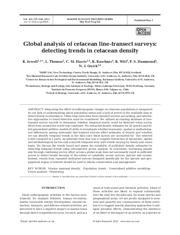Model 2 was used to generate predictions of temporal trends in cetacean density for those familyocean combinations with statistically significant smooth terms; those trends are shown in Fig. 1. The smooth term was highly significant for family Monodontidae in the Pacific and Balaenopteridae in the Atlantic (p ≤ 0.001, Table 3) suggesting density varied over time. Table 2. Details of the 5 final global models including the measures of goodness of fit — the generalised cross–validation (GCV) and Akaike’s Information criterion (AIC) scores — used during model selection. ‘*’ denotes that the covariates were included as interactions in the model, ‘+’ denotes that the covariates were included as main effects, while ‘s’ denotes that the covariates were included in the model as smooth terms Model Covariates 1 2 3 4 5 Species*OceanAgency*MethodG0Corr*Season + s(Year*Family) Species*OceanAgency*MethodG0Corr*Season + s(Year*FamilyOcean) Species*OceanAgency*MethodG0Corr*Season + s(Lat) Species*OceanAgency*MethodG0Corr*Season + s(Year*Ocean) Species*OceanAgency*MethodG0Corr*Season*Decade No. parameters Delta GCV Delta % deviance AIC explained 199 208 195 195 564 0 0.0038 0.0153 0.0164 0.0356 3.77 1.06 23.87 24.93 0 81.22 81.60 80.74 80.72 83.06 Jewell et al.: Trends in cetacean abundance a Monodontidae in the Pacific 0.30 0.12 b 233 Balaenopteridae in the Atlantic 0.10 0.08 0.20 0.06 0.10 0.04 0.02 0.00 1992 0.10 1996 2000 1990 2004 d Ziphiidae in the Altantic c 1995 2000 2005 Delphinidae in the Pacific Predicted density 0.0015 0.08 0.06 0.0010 0.04 0.0005 0.02 0.0000 0.00 1990 e 1995 1990 2000 Monodontidae in the Atlantic 0.25 0.12 f 1995 2000 2005 Delphinidae in the Atlantic 0.20 0.08 0.15 0.04 0.10 0.05 0.00 1982 1986 1990 1990 1994 1995 2000 2005 Year Fig. 1. Predicted density of the 6 most statistically significant family-ocean combinations from model 2 with ± 1 standard error shown; (a) Monodontidae in the Pacific, (b) Balaenopteridae in the Atlantic, (c) Ziphiidae in the Atlantic, (d) Delphinidae in the Pacific, (e) Monodontidae in the Atlantic, and (f) Delphinidae in the Atlantic. Note that the scale of the y-axis differs among plots. For illustration, the most common set of values of the Species*OceanAgency*MethodG0Corr*Season interaction term were used for each family-ocean combination, for example, for Monodontidae in the Pacific all density estimates were from summer aerial surveys of beluga whales where g(0) was corrected for and the majority of surveys were conducted by NOAA, and density was predicted only for the years for which density estimates were available Fig. 1a suggests a non-linear decline in density of Monodontidae occurred between 1993 and 2004 in the Pacific, while predicted densities of Balaenopteridae (Fig. 1b) and Ziphiidae (p = 0.003, Fig. 1c) in the Atlantic increased over the time frame modelled. There was some evidence from the smoothing to suggest temporal variability in density of Delphinidae in the Pacific (p = 0.020), Monodontidae in 234 Mar Ecol Prog Ser 453: 227–240, 2012 Table 3. Approximate significance of the smooth terms from model 2 for familyocean combinations with >10 density estimates and density estimates from >1 decade. The population change index (∆) and 95% confidence interval of ∆ are also given for each family-ocean combination. A ∆ of 1 suggests density in 2001−2005 did not differ from density in 1991−1995 0.05) smooth trend terms had 95% confidence intervals on ∆ that did not encompass 1, providing evidence of temporal trends in density (Table 3). The smooth term p-values and confidence intervals test differSmooth term Estimated Fp∆ 95%CI(∆) Family and Ocean degrees of statistic value ent hypotheses: the p-value tests if freedom the smooth trend terms are significant while the confidence interval Monodontidae Pacific 1.943 9.424 < 0.001 0.151 0.05−0.33 on ∆ tests the hypothesis that mean Balaenopteridae Atlantic 1.000 12.226 < 0.001 1.897 1.31−2.65 smoothed density in the last 5 years Ziphiidae Atlantic 1.023 8.503 0.003 6.458 0.96−23.24 Delphinidae Pacific 1.000 5.462 0.020 0.734 0.56−0.96 is different from mean smoothed Monodontidae Atlantic 1.000 3.984 0.046 0.496 0.21−1.00 density in the first 5 years. The Delphinidae Atlantic 1.778 2.801 0.058 1.652 0.96−2.66 direction of trends suggested by Phocoenidae Atlantic 1.000 1.235 0.267 1.993 0.66−4.78 the confidence intervals are the Phocoenidae Pacific 1.000 1.197 0.274 3.318 0.50−12.11 Balaenopteridae Antarctic 1.000 0.697 0.404 0.825 0.46−1.39 same as those suggested by the Balaenopteridae Pacific 1.000 0.500 0.480 1.401 0.63−2.78 smooth terms, with the biggest Delphinidae Mediterranean 1.025 0.415 0.529 9.121 0.14−58.74 change being a decrease in the prePhyseteridae Atlantic 1.000 0.043 0.836 1.013 0.35−2.31 dicted density of Monodontidae in Physeteridae Pacific 1.000 0.020 0.888 1.272 0.35−3.41 the Pacific to between 0.05 and 0.33 of their initial density. the Atlantic (p = 0.046) and Delphinidae in the To demonstrate the probability of observing a speAtlantic (p = 0.058) (Table 3). A slight increase in cific population trend given the level of variability density was predicted for Delphinidae in the Atlantic about the trend estimates we plotted isolines of sta(Fig. 1f), while a decrease in density of Delphinidae tistical power against a range of rates of population in the Pacific (Fig. 1d) and density of Monodontidae change ∆ and CV(∆). The relationship between popin the Atlantic (Fig. 1e) was predicted. No evidence ulation change ∆, CV(∆) and statistical power is was found to suggest temporal trends could be shown in Fig. 2; the dashed lines indicate the level of detected for any of the other family-ocean combinaestimated variability in population change estimates tions for which we had sufficient data, but this should for different family-ocean combinations and the be considered in light of the power analysis results. resulting power to detect different population changes. Given the large values estimated for CV(∆) in most cases, power is low to detect anything but the Power analysis largest population changes. For example, with a Estimated CVs for the population change index were calculated from the Year*FamilyOcean term in model 2. The CVs varied from 0.14 to 3.09, with a mean of 0.74 (Table 4), and were used to investigate our power to detect population change. The metric of change used in the power analysis was a comparison of the mean smoothed density estimate from recent years (2001−2005) with mean smoothed density from earlier years (1991−1995), so power analysis was only conducted for family-ocean combinations with density estimates from before 1995 and after 2001. Three of the family-ocean combinations with significant (i.e. p-value < Table 4. Estimated CVs for the population change index ∆, in order of ascending CV, and the population (pop.) change detectable with statistical power of 0.8 for family-ocean combinations with density estimates from before 1995 and after 2001. A subset of these results is shown in Fig. 2 Family and Ocean Abbreviation Number density estimates Delphinidae Pacific Balaenopteridae Atlantic Delphinidae Atlantic Balaenopteridae Pacific Monodontidae Pacific Physeteridae Atlantic Phocoenidae Atlantic Physeteridae Pacific Phocoenidae Pacific Ziphiidae Atlantic Delphinidae Mediterranean D_Pa B_At D_At B_Pa M_Pa Phy_At Pho_At Phy_Pa Pho_Pa Z_At D_Me 146 223 191 85 18 30 51 14 104 16 13 CV(∆) Approx. pop. change detectable (%) 0.14 0.18 0.27 0.39 0.50 0.51 0.54 0.63 0.96 0.97 3.09 5.1 8.8 17.5 32.8 46.1 47.7 51.1 60.5 84.0 84.3 99.0 Jewell et al.: Trends in cetacean abundance 1.8 1.6 1.4 0.4 0.6 0.2 1.0 8 0. CV(Δ) 1.2 Pho_Pa 0.8 Phy_Pa 0.6 M_Pa B_Pa 1 0.4 D_At 0.2 D_Pa 0.0 0.1 0.2 0.3 0.5 0.8 1.5 2.5 4 5.5 8 Population change (Δ) Fig. 2. Power to detect population changes ranging from 0.1 to 8.5 given a range of CVs on the population change estimate. A sample of the family-ocean combinations is shown. (Abbreviations are given in Table 4) CV(∆) of 0.63 (as for Physeteridae in the Pacific), a population change of approximately 61%, would be detectable with a power of 0.8 (a common benchmark for acceptable level of power) over the duration of the study (calculated here using a 15 yr study period). At the lowest estimated CV(∆) of 0.14 for Delphinidae in the Pacific, very small population changes of the order of 0.95 or 1.05 (i.e. a 5% increase or decline over the 15 yr study period) would be observable with high power; conversely Delphinidae in the Mediterranean (not shown in Fig. 2) had an estimated CV(∆) of 3.09, and only a 99% increase or decrease in population size over the study period would be detectable with a power of 0.8. DISCUSSION We have used survey and abundance data extracted from an existing database (Kaschner et al. unpubl.) to determine whether it is possible to combine wide-ranging datasets and account for their varying attributes to evaluate the presence of trends in species abundance, and to determine whether there is sufficient power in this approach to detect trends. There are numerous examples in the literature of studies that have struggled to demonstrate the existence of an increasing or decreasing trend in 235 abundance for a specific species or population due to a lack of power in the available survey data (e.g. Taylor et al. 2007, Waring et al. 2009), or have shown through power analysis that many years of data collection would be required to detect a trend given specific circumstances, such as small population size (e.g. Taylor & Gerrodette 1993, Wilson et al. 1999, Thompson et al. 2000). The probability of detecting a change in abundance is strongly correlated with the number and precision of samples: when you have a reasonable number of samples, the variability associated with each estimate must be low and the rate of change high to detect trends (Gerrodette 1987). Here, we wanted to determine whether combining survey data and correcting for any underlying patterns would give sufficient power to detect trends or whether the variability among surveys (temporal, geographical, taxonomic, and methodological) would confound any such trends. One aim of the analysis was to identify and detect generic biases arising from methodological factors that may impact our ability to detect trends in abundance using data collected during different surveys. The models suggest that survey season, ocean basin, research group, and g(0) correction affect density estimates differently for different species. Given the highly migratory nature of many species and the seasonal and geographical variation in habitat suitability, prey availability and impacts of anthropogenic activities, the variation in cetacean density with seasons and ocean basin can be expected. Similarly, accounting for those animals missed on the trackline (i.e. g(0) correction) should result in higher density estimates, and the level of increase was expected to vary among species because the detectability of different species varies substantially due to physiological and ecological differences. Our finding that density estimates are affected by research group, however, was less expected, although it is difficult to assess the extent of the research group effort due to possible confounding with spatial, temporal and other factors. For example, the SCANS surveys produced higher density estimates of 2 species of Delphinidae in the Atlantic than other surveys conducted in the Atlantic. However, the difference in estimated density cannot be attributed to the research group alone because the surveys were also conducted in different areas of the Atlantic and in different years. Interaction terms in the models made it difficult to quantify the individual effect of these factors on density and therefore to estimate correction factors for the potential sources of bias (i.e. survey agency and g(0) correction). Our inability to cor- 236 Mar Ecol Prog Ser 453: 227–240, 2012 rect for these sources of bias means that studies should be conducted at the species level, and data from well-studied (data-rich) species cannot be used to hypothesise about which factors may affect density estimates of data-poor species when estimating global trends. Moreover, we cannot estimate a single correction factor that could be applied across surveys and abundance estimates outside of this dataset. Nevertheless, the inclusion of the interaction term in the model means that we can interpret the current model outputs for the Year*FamilyOcean smooth term knowing that the variability in surveys has been accounted for. Despite this, we could not test whether factors affect trends at the species level because temporal trends were most parsimoniously modelled at the family level. Therefore, family level trends cannot be assumed to apply to species for which we had no data and neither can family level trends be assumed to reflect trends of individual species within the family for which data did exist within the database. For example, model 2 estimated a slight decline in density for those species of Delphinidae in the Pacific that were included in our dataset. There is published evidence of non-recovery of 2 populations of the species included in our dataset, the pantropical spotted dolphin Stenella attenuata attenuata and spinner dolphin Stenella longirostris orientalis, following a decline in abundance as a result of bycatch in the yellowfin tuna fishery in the eastern tropical Pacific Ocean (Gerrodette & Forcada 2005). Whilst it is encouraging that our model results are in agreement with other studies we must bear in mind that S. attentuata attentuata and S. longirostris orientalis are only 2 of 10 species of Delphinidae in the Pacific Ocean included in our analysis, and therefore we cannot make a direct link between our family level trend and these reported species level trends. In addition, a decline in abundance cannot be assumed to have occurred for those species of Delphinidae for which we did not have data from the Pacific, and without additional evidence the decline in abundance also cannot be assumed to apply to each of those 8 species of Delphinidae for which we did have density data from the Pacific. Unfortunately family level trends are unlikely to be useful in directly informing management decisions because management usually occurs at the stock level. The exception to this, however, is for the families Monodontidae and Physeteridae, as only one species from these families were represented in the analysis. Here, a decline in the abundance of beluga (Delphinapterus leucas, family Monodontidae) was estimated by model 2 which is consistent with what has been described. The non-linear decline in beluga density over time in the Pacific relates to 18 density estimates produced from aerial surveys conducted between 1992 and 2004 in Cook Inlet, Alaska (Hobbs et al. 2000, Rugh et al. 2005) and was described by Rugh et al. (2010). This decline, and range contraction, is thought to have resulted from unregulated subsistence hunting (Rugh et al. 2010). The hunt was suspended in 1999 and has been resumed at regulated low levels since then, but there has been no evidence of an increase in beluga abundance (Rugh et al. 2010). Estimated density from our model continued to decline following the suspension of hunting in 1999 (Fig. 1a). That all data for Monodontidae in the Pacific came from the same inlet was likely a contributing factor to the detection of the trend. On the other hand, we found no evidence of a temporal trend in the density of the Physeteridae family, which contains only one species, the sperm whale Physeter macrocephalus. The sperm whale data had good temporal coverage in both the Atlantic (30 density estimates from 1989 to 2004) and the Pacific (14 density estimates from 1988 to 2002); despite this, no evidence was found to suggest a temporal trend in sperm whale abundance in either ocean. This could represent a genuine lack of trend in sperm whales in both oceans, or that the combined survey estimates gave low statistical power to detect changes in abundance over time, or a combination of the two. Despite the fact that sperm whale populations worldwide were depleted from the early 18th century until 1988 (Whitehead 2002), direct evidence of populationlevel recovery since whaling ceased has not been found (Taylor et al. 2008). Ten years since modern whaling ceased, the global population was estimated to be 32% (95% CI: 19 to 62%) of its original, prewhaling level (Whitehead 2002). While it is possible that there is no trend in abundance for sperm whales in the Atlantic and Pacific, we had poor power to detect a trend should one exist. A population change of approximately 48% over the duration of the study period would be detectable with statistical power 0.8 for Physeteridae in the Atlantic, while a change of 61% would be detectable for Physeteridae in the Pacific. Our power analysis suggests population changes greater than these are unlikely to have occurred during the study period. Stock structure of a population and spatial scale of surveys are important considerations when looking for temporal trends in abundance; this will vary among species and populations. The same applies to the spatial scale at which we are able to model. Being able to consider a smaller spatial scale than ocean Jewell et al.: Trends in cetacean abundance basin may increase the likelihood of detecting trends but would require substantially more data to incorporate a further spatial covariate in this type of global analysis. Combining the Family and Ocean covariates made sense for detecting trends, as families occupying different oceans will experience different physical, biological and anthropogenic conditions and are therefore likely to demonstrate different abundance trends. For example, while North Pacific right whales Eubalaena japonica and North Atlantic right whales Eubalaena glacialis are severely threatened (Reilly et al. 2008a, Wade et al. 2009), southern right whales Eubalaena australis in the Atlantic are increasing (Reilly et al. 2008b). However, considering trends at the ocean level means differences in trend within a family in the same ocean would not be detectable and could in fact prevent any trend in abundance being detected. Had data from the Bristol Bay stock of belugas been included in the analysis in addition to data from the Cook Inlet stock, a decline in density may not have been predicted because an increasing trend in abundance has been observed in the Bristol Bay stock (Lowry et al. 2008, NMFS 2008). Modelling temporal data and including explanatory covariates to reduce ‘noise’ in the data that could obscure trends was one of the approaches to detecting declines in abundance suggested by Taylor et al. (2007). The current study has shown that increasing sample size through combining survey effort across a global scale does not necessarily result in sufficient power to detect trends. Variability in precision associated with estimates combined with variability in the size of study areas greatly reduced the effective sample size of the database. Further uncertainty was associated with the use of parameter estimates from the final model in the power analysis, the outcome of which was affected by the fit of the model to the data. These factors combined to give poor power to detect trends for most family-ocean combinations. The use of stepwise regression in ecology has been criticised on the basis that model selection algorithms are used inconsistently, multiple hypothesis testing occurs, attention is often focused on a single final model, and parameter estimates may be biased (Whittingham et al. 2006). Those who criticise null hypothesis testing during stepwise regression often advocate an information theoretic (IT) approach (Burnham & Anderson 2002) which encourages the a priori selection of competing models following careful consideration of likely hypotheses. All possible models in the model space are fitted to the data and selection criteria (often the AIC) are used to select the best model, or set of models. Weighting each 237 model according to its AIC score and model averaging provides more robust parameter estimates and model predictions by reducing model selection bias and accounting for model selection uncertainty (Johnson & Omland 2004, Nakagawa & Freckleton 2011). A full IT approach could not be implemented here because imbalances in the data prevented some models in the model space being fitted. Consequently, the possibility that a different combination of parameters could have a similarly good fit to the data cannot be excluded. Adjusting the fit of the model to the data during the stepwise approach also increased the chance of observing overestimated effect sizes in the final model (Hegyi & Garamszegi 2011). However, our approach did avoid the use of significance values of null hypothesis tests for model selection by using continuous model selection criteria (e.g. the AIC and GCV score), which provided a relative measure of fit for each of the models. These measures could have been used for model averaging (i.e. to weight a set of the ‘best’ models) to generate predictions and to form the basis of the power analysis, but the validity of model averaging in the presence of interaction terms ‘needs more attention’ (Hegyi & Garamszegi 2011). In summary, the stepwise regression method used here is not without its limitations, but it was deemed most suitable, given the aims of the analysis and the limitations of the available data. We have demonstrated with this dataset that confounding factors make it difficult to neatly categorise and account for the large amount of variability in abundance estimates derived from line-transect surveys. This conclusion highlights the need for dedicated cetacean surveys to be conducted as robustly as possible to minimise the variability associated with abundance estimates. Repeated dedicated surveys in the eastern tropical Pacific have demonstrated good statistical power to detect trends in abundance (Gerrodette & Forcada 2005) as have co-ordinated international North Atlantic sighting surveys (e.g. Pike et al. 2009a, Pike et al. 2009b, Víkingsson et al. 2009). These surveys, and others, are highly valuable and generally answer the questions they were designed to address. Whilst it was worth investigating, combining abundance estimates from multiple different surveys in order to address broader research questions generally resulted in poor statistical power to detect trends. This approach is unlikely to yield sufficiently sound results to reliably inform conservation or management decisions but may be the only option when long-term data from repeated surveys are lacking and should therefore be considered to make best Mar Ecol Prog Ser 453: 227–240, 2012 238 use of the available data. A Bayesian approach to ➤ Hegyi G, Garamszegi LZ (2011) Using information theory as a substitute for stepwise regression in ecology and betrend detection, similar to that of Moore & Barlow havior. Behav Ecol Sociobiol 65:69−76 (2011) might have had greater power to discern Heide-Jørgensen MP, Borchers DL, Witting L, Laidre KL, trends, and this approach should be explored. Simon MJ, Rosing-Asvid A, Pike DG (2008) Estimates of Acknowledgements. We are grateful to M. Lonergan for statistical advice and members of the International Association of Oil & Gas Producers (OGP), Joint Industry Program (JIP) for constructive comments. We also gratefully acknowledge the help of 2 anonymous reviewers for providing comments on the manuscript. Financial support for this project was provided by the OGP JIP E&P Sound and Marine Life Program under contract reference JIP22 06-10: Cetacean stock assessment in relation to Exploration and Production industry sound. ➤ LITERATURE CITED ➤ ➤ ➤ ➤ ➤ ➤ ➤ ➤ ➤ Barlow J (2003) Cetacean abundance in Hawaiian waters during summer/fall of 2002. Administrative Report LJ03-13. NOAA Southwest Fisheries Science Centre, La Jolla, CA Barlow J (2006) Cetacean abundance in Hawaiian waters estimated from a summer/fall survey in 2002. Mar Mamm Sci 22:446−464 Barlow J, Taylor BL (2005) Estimates of sperm whale abundance in the northeastern temperate Pacific from a combined acoustic and visual survey. Mar Mamm Sci 21: 429−445 Branch TA, Butterworth DS (2001) Southern hemisphere minke whales: standardized abundance estimates from the 1978/79 to 1997/98 IDCR/SOWER surveys. J Cetacean Res Manag 3:143−174 Buckland ST, Breiwick JM (2002) Estimated trends in abundance of eastern Pacific gray whales from shore counts (1967/68 to 1995/6). J Cetacean Res Manag 4:41−48 Burnham KP, Anderson DR (2002) Model selection and multimodel inference: a practical information-theoretic approach, 2nd edn. Springer, New York, NY Galimberti F (2002) Power analysis of population trends: an application to elephant seals of the Falklands. Mar Mamm Sci 18:557−566 Gerrodette T (1987) A power analysis for detecting trends. Ecology 68:1364−1372 Gerrodette T, Forcada J (2005) Non-recovery of two spotted and spinner dolphin populations in the eastern tropical Pacific Ocean. Mar Ecol Prog Ser 291:1−21 Gibbs JP, Droege S, Eagle P (1998) Monitoring populations of plants and animals. Bioscience 48:935−940 Gilles A, Scheidat M, Siebert U (2009) Seasonal distribution of harbour porpoises and possible interference of offshore wind farms in the German North Sea. Mar Ecol Prog Ser 383:295−307 Gómez de Segura A, Hammond PS, Cañadas A, Raga JA (2007) Comparing cetacean abundance estimates derived from spatial models and design-based line transect methods. Mar Ecol Prog Ser 329:289−299 Hammond PS, Berggren P, Benke H, Borchers DL and others (2002) Abundance of harbour porpoise and other cetaceans in the North Sea and adjacent waters. J Appl Ecol 39:361−376 Hastie TJ, Tibshirani RJ (1990) Generalised additive models. Chapman & Hall, London ➤ ➤ ➤ ➤ ➤ ➤ large whale abundance in West Greenland waters from an aerial survey in 2005. J Cetacean Res Manag 10:119−129 Hobbs R, Rugh D, DeMaster D (2000) Abundance of beluga whales, Delphinapterus leucas, in Cook Inlet, Alaska, 1994−2000. Mar Fish Rev 62:37−45 Hoenig JM, Heisey DM (2001) The abuse of power: the pervasive fallacy of power calculations for data analysis. Am Stat 55:19−24 James FC, McCulloch CE, Wolfe LE (1990) Methodological issues in the estimation of trends in bird populations with an example: the pine warbler. In: Sauer JR, Droege S (eds) Survey designs and statistical methods for the estimation of avian population trends. Biological Report 90(1). U.S. Fish and Wildlife Service, Washington, DC Jefferson TA, Webber MA, Pitman RL (2008) Marine mammals of the world: a comprehensive guide to their identification. Elsevier, London Johnson JB, Omland KS (2004) Model selection in ecology and evolution. Trends Ecol Evol 19:101−108 Laake JL, Calambokidis JC, Osmek SD, Rugh DJ (1997) Probability of detecting harbor porpoise from aerial surveys: estimating g(0). J Wildl Manag 61:63−75 Lowry LF, Frost KJ, Zerbini A, DeMaster D, Reeves RR (2008) Trends in aerial counts of beluga or white whales (Delphinapterus leucas) in Bristol Bay, Alaska, 1993− 2005. J Cetacean Res Manag 10:201−207 Marques TA, Thomas L, Ward J, DiMarzio N, Tyack PL (2009) Estimating cetacean population density using fixed passive acoustic sensors: an example with Blainville’s beaked whales. J Acoust Soc Am 125:1982−1994 Mollett A, Schofield C, Miller I, Harwood J, Harris C, Donovan C (2009) Environmental risk management capability: advice on minimizing the impact of both sonar and seismic offshore operations on marine mammals. Proc SPE Offshore Europe Oil and Gas Conference, Aberdeen Moore JE, Barlow J (2011) Bayesian state-space model of fin whale abundance trends from a 1991−2008 time series of line-transect surveys in the California Current. J Appl Ecol 48:1195−1205 Nakagawa S, Freckleton RP (2011) Model averaging, missing data and multiple imputation: a case study for behavioural ecology. Behav Ecol Sociobiol 65:103−116 National Marine Fisheries Service (2008) Beluga whale (Delphinapterus leucas): Bristol Bay stock. Stock Assessment Report, p 77−81 Parra GJ, Corkeron PJ, Marsh H (2006) Population sizes, site fidelity and residence patterns of Australian snubfin and Indo-Pacific humpback dolphins: implications for conservation. Biol Conserv 129:167−180 Pike DG, Paxton CGM, Gunnlaugsson Th, Víkingsson GA (2009a) Trends in the distribution and abundance of cetaceans from aerial surveys in Icelandic coastal waters, 1986–2001. NAMMCO Sci Publ 7:117−142 Pike DG, Vikingsson GA, Gunnlaugsson Th, Øien N (2009b) A note on the distribution and abundance of blue whales (Balaenoptera musculus) in the Central and Northeast North Atlantic. NAMMCO Sci Publ 7:19−29 R Development Core Team (2008) A language and environment for statistical computing. R Foundation for Statistical Computing, Vienna, Austria. www.R-project.org Jewell et al.: Trends in cetacean abundance ➤ ➤ ➤ ➤ ➤ Reilly SB, Bannister JL, Best PB, Brown M and others (2008a) Eubalaena glacialis. In: IUCN 2010. IUCN Red List of Threatened Species. Version 2010.4. Accessed 02 June 2011. www.iucnredlist.org Reilly SB, Bannister JL, Best PB, Brown M and others (2008b) Eubalaena australis. In: IUCN 2010. IUCN Red List of Threatened Species. Version 2010.4. Accessed 08 Dec 2010. www.iucnredlist.org Rugh D, Shelden K, Sims C, Mahoney B, Smith B, Litzky L, Hobbs R (2005) Aerial surveys of belugas in Cook Inlet, Alaska, June 2001, 2002, 2003, and 2004. NOAA Tech Memo NMFS-AFSC-149, Seattle, WA Rugh DJ, Sheldon KEW, Hobbs RC (2010) Range contraction in a beluga whale population. Endang Species Res 12: 69−75 SCANS-II (2008) Small cetaceans in the European Atlantic and North Sea. Final report to the European Commission under project LIFE04NAT/GB/000245. http://biology.standrews.ac.uk/scans2/inner-finalReport. html Schipper J, Chanson JS, Chiozza F, Cox NA and others (2008) The status of the world’s land and marine mammals; diversity, threat, and knowledge. Science 322: 225−230 Smith TD, Allen J, Clapham PJ, Hammond PS and others (1999) An ocean-basin-wide mark-recapture study of the North Atlantic humpback whale (Megaptera novaeangliae). Mar Mamm Sci 15:1−32 Steidl RJ, Thomas L (2001) Power analysis and experimental design. In: Scheiner S, Gurevitch J (eds) Design and analysis of ecological experiments. Oxford University Press, New York, p 14–36 Taylor BL, Gerrodette T (1993) The uses of statistical power in conservation biology: the vaquita and northern spotted owl. Conserv Biol 7:489−500 Taylor BL, Martinez M, Gerrodette T, Barlow J, Hrovat YH (2007) Lessons from monitoring trends in abundance of marine mammals. Mar Mamm Sci 23:157−175 Taylor BL, Baird R, Barlow J, Dawson SM and others (2008) Physeter macrocephalus. In: IUCN 2010. IUCN Red List of Threatened Species. Version 2010.4. Accessed 03 Dec 2010. www.iucnredlist.org 239 ➤ Thomas L (1997) Retrospective power analysis. Conserv Biol ➤ ➤ ➤ ➤ ➤ ➤ 11:276−280 Thompson PM, Wilson B, Grellier K, Hammond PS (2000) Combining power analysis and population viability analysis to compare traditional and precautionary approaches to conservation of coastal cetaceans. Conserv Biol 14:1253−1263 Víkingsson GA, Pike DG, Desportes G, Øien N, Gunnlaugsson Th, Bloch D (2009) Distribution and abundance of fin whales (Balaenoptera physalus) in the Northeast and Central Atlantic as inferred from the North Atlantic Sightings Surveys 1987−2001. NAMMCO Sci Publ 7: 49−72 Wade P, Kennedy AS, LeDuc RG, Barlow J and others (2009) First abundance estimates for eastern North Pacific right whales (Eubalaena japonica) using mark-recapture methods applied to both genetic and photo-identification data. Proceedings of the 18th biennial conference on the biology of marine mammals, Quebec Waring GT, Josephson E, Maze-Foley K, Rosel PE (2009) U.S. Atlantic and Gulf of Mexico marine mammal stock assessments — 2009. NOAA Tech Memo NMFS-NE213 Whitehead H (2002) Estimates of the current global population size and historical trajectory for sperm whales. Mar Ecol Prog Ser 242:295−304 Whittingham MJ, Stephens PA, Bradbury RB, Freckleton RP (2006) Why do we still use stepwise modeling in ecology and behaviour? J Anim Ecol 75:1182−1189 Wilson B, Hammond PS, Thompson PM (1999) Estimating size and assessing trends in a coastal bottlenose dolphin population. Ecol Appl 9:288−300 Wood SN (2006) Generalized additive models. An instruction with R. Chapman & Hall, London Wood SN (2008) Fast stable direct fitting and smoothness selection for generalized additive models. J R Stat Soc B 70:495−518 Zeh JE, George JC, Raftery AE, Carroll GM (1991) Rate of increase, 1978−1988, of bowhead whales, Balaena mysticetus, estimated from ice-based census data. Mar Mamm Sci 7:105−122 Mar Ecol Prog Ser 453: 227–240, 2012 240 Appendix 1. Supplementary tables and diagnostic plots of model 2 Family No. Species included fam. No. est. 2 Deviance residuals Table A1. Representative species from each family (No. fam. = number of species in the family) and number of abundance estimates (No. est.) used in the analysis. Species names match those of Jefferson et al. (2008) 1 0 -1 -2 Delphinidae 33 Balaenopteridae 8 Physeteridae Monodontidae 1 2 Harbour porpoise Dall’s porpoise Short-beaked common dolphin Long-finned pilot whale Risso’s dolphin Atlantic white-sided dolphin White-beaked dolphin Pacific white-sided dolphin Northern right whale dolphin Killer whale Pantropical spotted dolphin Rough-toothed dolphin Striped dolphin Atlantic spotted dolphin Spinner dolphin Common bottlenose dolphin Common minke whale Sei whale Blue whale Fin whale Humpback whale Northern bottlenose whale Cuvier’s beaked whale Sperm whale Beluga 75 83 30 29 32 21 10 22 15 32 25 10 31 17 18 63 112 27 12 92 83 11 11 48 57 -4 -2 0 2 Theoretical quantiles Histogram of residuals 200 Frequency 6 100 50 0 -2 -1 1 0 Residuals 2 Resids vs. linear pred. 2 Residuals Phocoenidae 1 0 -1 -2 Table A2. Groupings for explanatory covariate OceanAgency used in the analysis. NOAA: US National Oceanic and Atmospheric Administration, includes all National Marine Fisheries Science Centres, NASS: North Atlantic Sighting Survey, SCANS: Small Cetaceans in the European Atlantic and North Sea. Surveys conducted by other agencies were grouped into a single category Survey agency grouping Antarctic Arctic Arctic Atlantic Atlantic Atlantic Atlantic Indian Ocean Mediterranean Pacific Pacific Other agencies NOAA Other agencies NASS NOAA Other agencies SCANS Other agencies Other agencies NOAA Other agencies Editorial responsibility: Matthias Seaman, Oldendorf/Luhe, Germany -8 -6 -4 -2 Linear predictor 0 Response vs. Fitted values 2.5 Response Survey ocean -10 2.0 1.5 1.0 0.5 0 0.0 0.5 1.0 1.5 Fitted values 2.0 Fig. A1. Diagnostic plots for model 2. From top: (a) quantile–quantile plot, (b) histogram of residuals, (c) model residuals plotted against fitted values, (d) response variable plotted against fitted values Submitted: July 29, 2011; Accepted: January 31, 2012 Proofs received from author(s): April 27, 2012