2014 American Control Conference (ACC) June 4-6, 2014. Portland, Oregon, USA Cross-coupling Effect Compensation of an AFM Piezoelectric Tube Scanner for Improved Nanopositioning M. S. Rana, Student Member, IEEE, H. R. Pota, Member, IEEE, and I. R. Petersen, Fellow, IEEE Abstract—The imaging performance of an atomic force microscope (AFM) at high scanning speeds is limited due to the crosscoupling properties of its scanning unit; i.e., the piezoelectric tube scanner (PTS). In order to increase the imaging speed of an AFM, a multi-input multi-output (MIMO) model predictive control (MPC) scheme is used for the PTS to reduce its crosscoupling effect. The design of this controller is based on an identified MIMO model of the AFM PTS. Also, a damping compensator is designed and included in the feedback loop with the plant to suppress the vibration of the PTS at the resonant frequency. Experimental results confirm the efficacy of the proposed controller. I. I NTRODUCTION The atomic force microscope (AFM) invented by Binnig et al. [1] is a unique invention capable of capturing highresolution images of samples in different environment. It enables precise control, manipulation, and interrogation of matter at nanoscale [2]. It has the ability to generate threedimensional images of material surfaces at an extremely high resolution down to the atomic level (10−10 m). It is extensively used in areas such as nanolithiography, DNA nanotechnology, optics, microelectronics, material science, and nanofabrication [3]–[7]. It has high spatial resolution, but a low temporal resolution, i.e., its imaging is slow, e.g., an image frame of a living cell takes 1-2 minutes and this means that rapid biological processes that occur in seconds cannot be studied using the commercially available AFMs. Fast and precise positioning is a basic requirement for nanotechnology applications. Many AFMs use a piezoelectric tube scanner (PTS) for actuation with nano-meter resolution in all three spatial directions. Due to the dynamics of the PTS, the imaging speed of the AFM is limited. The most prominent limitations of the PTS are the low mechanical resonance frequency [8], cross coupling between the axes [9], and non-linear behavior in the form of hysteresis and creep effects [10]. The lightly damped resonant modes in the PTS create significant distortions in the AFM’s scanned images. To suppress the resonant mode of the PTS, a positive velocity and position feedback (PVPF) controller is proposed by Bhikkaji et al. in [11]. The fast axis, i.e., the X-axis of the PTS is driven by a triangular signal and the slow axis, i.e., the Y -axis is driven by a slowly increasing staircase signal or the ramp signal [12]. This triangular signal contains odd harmonics of the fundamental frequency excite the resonance of the PTS due to which the images at high scanning rates are distorted. To solve the triangular reference signal problem a spiral scanning method with improved control is proposed in [7]. The effectiveness of the spiral trajectory scheme over that of the conventional raster positioning pattern is examined in [13] by applying it to a MEMS-based scanning-probe data-storage setup for thermo-mechanical storage on a polymer medium. Cycloid scanning is another scanning method which is introduced in [14]. In [15] an alternative non-raster scan method, based on Lissajous pattern, which allows faster operations compared to the ordinary scan patterns, is introduced. One of the important problems in AFM imaging is the cross-coupling effect between the axes of the PTS. The crosscoupling effect between the axes of the PTS introduces a significant amount of error in the high-speed precision positioning of the PTS. Due to this effect, the signal applied to the any of the axes of a PTS results in displacements in both axes of the scanner and introduces artifacts on scanned images. To compensate for the cross-coupling effect of a PTS in tappingmode AFM imaging, an inversion-based iterative control (IIC) method is proposed in [16]. Although this technique works well for cross-coupling compensation, it only produces good quality scanned images up to 24.4 Hz scanning speed. Improved mechanical design of the scanner can also limit the cross-coupling effect. In [17], a novel flexure-based piezoelectric stack-actuated XY nanopositioning stage is presented which significantly reduces the cross-coupling effect and combined with integral resonant control (IRC) and feedforward control techniques, accurate high-speed scans up to 400 Hz were achieved. Nonlinearities in the form of hysteresis and creep effects are also responsible for limiting the performance of the AFM, with the former prominent during large scanning operations and the latter when scanning is performed over an extended period of time. In [18] a scheme is proposed to solve these problems using a single-input single-output (SISO) model predictive control (MPC) and achieved a significant improvement against hysteresis and creep effect but the cross-coupling effect between the axes of its PTS limited the high-speed scanning performance. M. S. Rana, H. R. Pota, and I. R. Petersen are with the School of Engineering and Information Technology (SEIT), The University of New South Wales, Canberra, ACT 2600, Australia (e-mail: m.rana@student.unsw.edu.au; h.pota@adfa.edu.au; i.petersen@adfa.edu.au). This work was supported by the Australian Research Council. 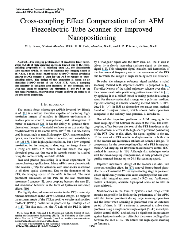978-1-4799-3274-0/$31.00 ©2014 AACC 2456 DSA 20 ADC dSPACE DAC 1103 Magnitude (dB) Magnitude (dB) 20 10 0 −10 −20 1 10 2 10 0 −20 −40 −60 −80 1 10 3 10 HVA -Y dx Measured open−loop Identified model 10 2 10 −20 −40 1 10 3 Frequency (Hz) SAM Measured open−loop Identified model 10 2 10 3 Frequency (Hz) +Y (a) Gxx Z AFM PTS (b) Gxy Magnitude (dB) 20 Fig. 1. Block diagram of the experimental setup (ADC is analog to digital converter and DAC is digital to analog converter). 0 −20 −40 −60 1 10 A. Contribution of This Work 20 Magnitude (dB) -X +X 3 0 10 2 10 3 10 0 −10 −20 1 10 The main contribution of this article is the utilization of a multi-input multi-output (MIMO) MPC scheme with a damping compensator to compensate for cross-coupling effects of the PTS to achieve improved nanopositioning. Using the MPC scheme proposed in this paper, it is possible to constrain the control signal within allowable range of the PTS. Since MPC is designed according to the linear PTS model, the control signal computation is less complicated than that using the nonlinear MPC. The augmented integral action of the MPC controller reduces the nonlinear behavior of the PTS which, in turn, solves the tracking error problem and a Kalman filter is used to obtain full state information of the system. The remainder of this paper is organized as follows: The experimental setup used for the present work is described in Section II. The identification and modeling of the PTS using a system identification method is presented in Section III. The design and selection of the controller are shown in Section IV, while Section V presents the performance of the proposed controller. Finally, the paper is concluded with brief remarks in Section VI. II. E XPERIMENTAL S ETUP The experimental setup at the University of New South Wales (UNSW), Canberra, Australia, consists of an NT-MDT Ntegra scanning probe microscope (SPM), configured to operate as an AFM. It contains a signal access module (SAM), control electronics, vibration isolator, computer for operating the AFM NOVA software, and other accessories, that is, a dynamic signal analyzer (DSA), a DSP dSPACE RT-1103, and a high-voltage amplifier (HVA) with a constant gain of 15 for supplying power to the X, Y , and Z-piezos using the SAM as an intermediate device. In this work, a Sm8133cl type scanner is used which is a “scan by head” type of scanner. The scanning range of this scanner in (X, Y , Z) is 100 µm × 100 µm × 10 µm and resonance frequencies in both the x and y directions of approximately 700-800 Hz and in the z direction of about 5 kHz. A block diagram of the experimental setup is shown in Fig. 1. Phase (rad) 10 0 −10 −20 1 10 2 10 10 3 4 Phase (rad) Capacitive sensor 0 −5 1 10 10 20 Phase (rad) Phase (rad) 5 2 10 Measured open−loop Identified model 10 2 10 3 2 0 −2 1 10 Measured open−loop Identified model 2 10 Frequency (Hz) Frequency (Hz) (c) Gyx (d) Gyy 10 3 Fig. 2. Frequency responses of the measured and identified systems for (a) input to the X-piezo and output from the X position sensor, (b) input to the Y -piezo and output from the X position sensor, (c) input to the X-piezo and output from the Y position sensor, and (d) input to the Y -piezo and output from the Y position sensor. III. I DENTIFICATION OF THE PTS DYNAMICS A PTS is the most useful actuator in nanopositioning applications, e.g., microscopes, and is made of ceramic lead zirconate and titanate (PZT). It consists of a tube of radially poled piezoelectric material, four external electrodes and a grounded internal electrode. The dynamics of the PTS can be modeled either using conventional mathematical theory or using an experimental approach. In the present work, we have used an experimental approach to model the AFM lateral positioning system as a MIMO system. In this experiment, the plant is identified using a bandlimited random noise signal within the frequency range from 10 Hz to 1.0 kHz, using a dual channel HP35665A DSA. This signal is supplied to the HVA as an input and the corresponding amplified voltage is supplied to the SAM of the AFM from which there is a direct connection to the PTS. The output displacement of the PTS is taken from the capacitive position sensor. The sensor output is fed back to the DSA to obtain frequency response functions (FRFs). The FRFs generated in the DSA are processed in MATLAB and using prediction error method (PEM), a system model is obtained. The best fit model frequency responses for the X and Y -piezos are shown in Fig. 2. The two inputs are the voltages applied to the x and y-axes amplifiers [vx , vy ]T while the corresponding output from the capacitive sensors [dx , dy ]T . 2457 R Vin Ci + Ai R Vout - - Damping Compensator + Ri ux Li Fig. 3. The FRFs of the AFM lateral positioning system can be described by the following equation [ ] Gxx (jω) Gxy (jω) Gdv (jω) = ; Gyx (jω) Gyy (jω) [ d (jω) d (jω) ] x = vx (jω) dy (jω) vx (jω) = AFM Signal Access Module vxref v yref ∑ ∑ AFM PTS Capacitive Sensor dx Capacitive Sensor dy ; (1) Fig. 5. Block diagram of the closed-loop system. vxref and vyref are the scanning reference waveforms provided by the AFM signal access module. The outputs dx and dy are the displacements of the tube scanner. −1.197×104 s3 −2.289×106 s2 +1.205×109 s−1.599×1013 s4 +3.859×105 s3 +6.626×107 s2 +1.806×1011 s+2.849×1013 ;(2) B. Design of MIMO MPC dx (s) vy (s) = dy (s) vx (s) = 4.242s3 −2460s2 +2.682×106 s−8.622×108 s4 +95.6s3 +1.016×106 s2 +4.498×107 s+2.56×1011 ; (3) 0.9309s3 −5498s2 +2.551×106 s−2.692×109 s4 +379.8s3 +9.67×105 s2 +1.772×108 s+2.327×1011 ; (4) The purpose of this section to present the design of an MIMO MPC controller for minimizing the cross-coupling effects in the AFM’s PTS. The construction of this closedloop system is shown in Fig. 5. The plant is described by the following state-space model: xm (k + 1) and dy (s) vy (s) MIMO MPC x vy (jω) dy (jω) vy (jω) where dx (s) vx (s) Feedback loop of the damping compensator for the X-piezo. Fig. 4. A structure of damping compensator. dx Plant (AFM PTS) å = −40.86s3 +2.703×104 s2 −1.363×107 s−6.895×1010 s4 +1.763×103 s3 +7.812×105 s2 +8.214×108 s+1.316×1011 .(5) IV. C ONTROLLER D ESIGN A. Design of Damping Compensator This section presents the design of a damping compensator, the basic structure of which is shown in Fig. 3. Although the MPC controller has itself some damping capacity, a damping compensator is introduced to achieve better damping of the resonant mode and higher bandwidth for an AFM’s PTS, and its feedback loop for the X-piezo is shown in Fig. 4. The general form of the damping compensator is [19]: Ai = N ∑ i=1 −ki Ci s(Ri + Li s) ; Li Ci s 2 + R i Ci s + 1 Am xm (k) + Bm u(k); (7) Cm xm (k) + Dm u(k); (8) Am , Bm , Cm , and Dm define the discrete state-space plant model, derived from the identified plant model, as stated in Eqs. (2)-(5) and Eq. (6) at a sampling time Ts , u = [vx , vy ]T is the manipulated variable or input variable, y = [dx , dy ]T is the measured output, and xm is the state variable vector with a dimension of n. Due to the principle of receding horizon control, where current information of the plant is required for prediction and control, we have implicitly assumed that the input u(k) cannot affect the output y(k) at the same time and hence the feedthrough term, Dm = 0. In order to incorporate integral action for disturbance rejection and tracking a reference signal in the MPC algorithm, the plant can be augmented in the following way [20]: x(k+1) z [ (6) where i = 1, 2, · · · , N , ki is the compensator gain of the corresponding mode. By selecting the proper value of Li , Ri , and Ci , we are able to improve damping of the resonant mode of the PTS. Since ωi = √L1 C , the value of Li and Ci are chosen such i i that ωi is equal to or almost equal to the resonant frequency of the system. = y(k) = }| ]{ ∆xm (k + 1) y(k + 1) x(k) A = z [ }| 0 I Am Cm Am B + z[ ]{ z[ }| ]{ ∆xm (k) y(k) }| ]{ Bm ∆u(k); Cm Bm (9) x(k) C y(k) = z[ }| z ]{ {] [ ∆xm (k) 0 I ; y(k) }| where A, B, and C are the augmented system matrices. 2458 (10) −40 1 10 2 3 10 10 0 −5 Measured closed−loop Measured open−loop −10 1 10 −0.04 −0.04 10 2 0 −20 −0.06 10 2 Magnitude (dB) 0 −50 2 3 10 10 10 −40 1 10 2 0.08 10 + 2 3 10 Frequency (Hz) 10 −10 1 10 2 3 10 Frequency (Hz) 10 (d) The output sequence for Np , prediction horizon can be written as: Y = F x(k) + Φ∆U ; (11) y(k + Np |k)        ; ∆U =    ∆u(k) ∆u(k + 1) .. . ∆u(k + Nc − 1)    .  CANp −2 B ··· ··· umin ≤ u(k + i − 1) ≤ umax , i = 1, . . . , Nc ; (13a) ∆umin ≤ ∆u(k + i − 1) ≤ ∆umax , i = 1, . . . , Nc ; (13b) where Q is the state weighting matrix, R is the control weighting, Rs is the reference signal, umin and umax are the low and high levels of the control action, respectively, and ∆umin and ∆umax are the low and high levels of the control increments, respectively. By considering the above equations, the constrained MPC problem can be expressed as a quadratic programming (QP) problem: 1 (14) min( ∆U T H∆U + ∆U T f ); 2 s.t. M ∆U ≤ γ; where where Nc is the control horizon, and the F matrix with dimensions of (2Np , n) and the Φ matrix with dimensions of (2Np , 2Nc ) are:   CA  CA2    3   F =  CA  ;   ..   . Np CA   CB 0 ··· ··· 0   CAB CB ··· ··· 0     CA2 B CAB ··· ··· 0 Φ= .   .. .. . . . . . .   . . . . . CANp −1 B R(∆u(k + m − 1)) ; subject to the linear inequality constraints on the system inputs, i.e: Measured open−loop Measured closed−loop Fig. 6. Comparison of measured open-loop and closed-loop frequency responses for: (a) X-piezo, (d) Y -piezo and cross-coupling for X and Y sensor outputs (b) input to the Y -piezo, output from the X-piezo, (c) input to the X-piezo, output from the Y -piezo. y(k + 1|k) y(k + 2|k) .. . (12) 2 m=1 0 −5 Q(y(k + m|k) − Rs (k + m))2 m=1 Nc ∑ 3 10 (c)   Y =  0.04 0.06 Time (s) (b) Np ∑ J= −20 Phase (rad) Measured open−loop Measured closed−loop in which  0.02 cost function defined as: 0 5 0 −40 1 10 −0.08 0 Fig. 7. Cross-coupling properties of the scanner at 10.42 and 31.25 Hz, respectively [closed-loop (red) and open-loop (blue)]. 20 20 −20 0.2 (a) 3 10 Frequency (Hz) 0.1 0.15 Time (s) (b) 50 −100 1 10 0.05 Measured open−loop Measured closed−loop −40 1 10 3 10 Frequency (Hz) −0.08 0 (a) Magnitude (dB) 3 −0.02 20 Phase (rad) Phase (rad) 2 10 −0.06 5 Phase (rad) −0.02 y −50 −100 1 10 d (µm) −20 0 0 0 y 0 0.02 0.02 50 d (µm) Magnitude (dB) Magnitude (dB) 20 CANp −Nc B The control law is derived based on the minimization of the H = ΦT QΦ + R; f = ΦT QF x(k + 1|k) − ΦT QRs ; M ∈ Rmc ×2Nc and γ ∈ R2Nc ×1 are computed using Eq. (13), mc is the number of constraints and Rs ∈ R2Np ×1 is the reference signal. In this paper for constraint calculation the Hildreth’s QP algorithm has been considered. The constrained minimization over ∆U is given by ∆U = −H −1 (f + M T λ) (15) where λ is the Lagrange multiplier, which is calculated by using M , γ, H, and f . The Kalman state observer estimates the states from the measured output and dynamics are: x̂(k + 1) ŷ(k) = = (A − LC)x̂(k) + Bu(k) + Ly(k); (16) Ĉ x̂(k); (17) where x̂(k) is the estimated state, ŷ(k) is the estimated output, Ĉ is the identity matrix of dimension n × n, and L 2459 0 0.02 0.02 0 0 −0.01 d (µm) d (µm) −0.02 −0.02 x x −0.03 x d (µm) −0.02 −0.04 −0.06 0 −0.04 −0.04 −0.05 0.1 0.2 −0.06 0 0.3 Time (s) −0.06 0.02 0.08 0.1 0 (b) 0.12 0.08 0.08 0.08 0.04 0.04 0.04 0 x x d (µm) 0.12 0 −0.04 −0.04 −0.08 −0.08 −0.08 0.1 0.2 −0.12 0 0.3 Time (s) (d) 0.02 0.04 Time (s) 0.06 0 −0.04 −0.12 0 0.02 (c) 0.12 d (µm) dx(µm) (a) 0.04 0.06 Time (s) 0.04 0.06 Time (s) 0.08 −0.12 0 0.1 (e) 0.02 0.04 Time (s) 0.06 (f) −0.066 −0.028 −0.0695 −0.067 −0.029 −0.07 −0.03 −0.0705 −0.031 −0.071 −0.032 −0.0715 0.2 0.4 −0.072 0 0.6 Time (s) (a) −0.071 0 0.3 y −0.49 (c) −0.4 −0.37 −0.38 Time (s) (d) 0.6 −0.41 −0.42 −0.39 0.4 0.12 y d (µm) y −0.48 0.04 0.08 Time (s) −0.39 −0.36 0.2 −0.069 (b) −0.47 d (µm) 0.1 0.2 Time (s) −0.35 −0.46 −0.5 0 −0.068 −0.07 d (µm) −0.033 0 dy (µm) −0.069 dy (µm) −0.027 y d (µm) Fig. 8. Sub-figures (a)-(c) are open-loop and sub-figures (d)-(f) are closed-loop in the comparison of tracking performance of triangular waves at 10.42, 31.25, and 62.50 Hz, respectively. −0.4 0 0.1 0.2 Time (s) (e) 0.3 −0.43 0 0.04 0.08 Time (s) 0.12 (f) Fig. 9. Sub-figures (a)-(c) are open-loop and sub-figures (d)-(f) are closed-loop in the comparison of tracking performance of staircase waves at 10.42, 31.25, and 62.50 Hz, respectively. 2460 is the observer gain which depends on the Gaussian white noise, process noise covariance, and the measurement noise covariance. V. E XPERIMENTAL R ESULTS For the purpose of performance evaluation, the proposed controller is implemented on the AFM and a frequency domain analysis carried out by comparing the measured open-loop and closed-loop frequency responses and reductions in crosscoupling effect as shown in Fig. 6. Figure 6(a) and (d) show comparisons of the closed-loop frequency plots of the X and Y -piezos obtained by implementing the MIMO MPC controller with the damping compensator, which indicate that it achieves high closed-loop bandwidths and damping of the resonant mode for X and Y -piezo, respectively, and in turn, significantly reduces vibrations. In addition, there is a reasonable amount of reduction in the cross-coupling for the X and Y -piezos as shown in Fig. 6(b) and (c). It is noteworthy that the resonant mode in the both cases of the cross-coupling has been reduced significantly. Thus, the controller reduces oscillation and vibration in the system. It should be noted that, using the current experimental setup, it was not possible to measure the closed-loop frequency responses of the AFM scanner with the well-tuned built-in AFM PI controller. Figure 7(a) and (b) show comparisons of the open-loop and closed-loop cross-couplings for the 10.42 and 31.25 Hz input reference signals, respectively. They illustrate that there is a significant improvement in cross-coupling in the closed-loop. To measure this cross-coupling, a reference triangular signal is applied to the X-piezo, and the output is taken from the Y position sensor. The overall improvement in the nanopositioning of the AFM PTS using the proposed controller is clearly be seen from the resulting open-loop and closed-loop sensor output displacement for the triangular reference input signal in the X-piezo and staircase reference signal in the Y -piezo for scanning speeds at 10.42, 31.25, and 62.50 Hz are given in Fig. 8 and Fig. 9, respectively. Due to the uncontrolled tube resonance in the open-loop condition, the output of the sensor becomes distorted and this effect becomes extreme at high scanning speeds. On the other hand, the improvement in lateral positioning in the closed-loop condition the sensor outputs remain better than the open-loop condition even at high scanning speeds. VI. C ONCLUSION In this article, results from a study of the high-precision positioning of an AFM PTS using an MIMO MPC controller augmented with a damping compensator are reported. The closed-loop frequency-domain performance is compared with the open-loop frequency responses and is shown to achieve significant damping of the resonant mode of the PTSs and to reduce the cross-coupling effects between its axes. The experimental results show high-precision positioning performance of the proposed controller at high scanning speed. R EFERENCES [1] G. K. Binnig, C. F. Quate, and C. Gerber, “Atomic force microscope (AFM),” Physical Review Letters, vol. 56, no. 9, pp. 930–933, Mar. 1986. [2] B. J. Kenton, A. J. Fleming, and K. K. Leang, “Compact ultra-fast vertical nanopositioner for improving scanning probe microscope scan speed,” Review of Scientific Instruments, vol. 82, no. 12, pp. 123 703– 123 703–8, Dec. 2011. [3] M. S. Rana, H. R. Pota, and I. R. Petersen, “High-speed AFM image scanning using observer-based MPC-Notch control,” IEEE Transactions on Nanotechnology, vol. 12, no. 2, pp. 246–254, Mar. 2013. [4] E. Meyer, H. J. Hug, and R. Bennewitz, Scanning Probe Microscopy. Berlin, Germany: Springer-Verlag, 2004. [5] M. S. Rana, H. R. Pota, I. R. Petersen, and Habibullah, “Improvement of the tracking accuracy of an AFM using MPC,” in 8th IEEE Conference on Industrial Electronics and Applications, 2013, pp. 1681–1686. [6] Habibullah, H. R. Pota, I. R. Petersen, and M. S. Rana, “Creep, hysteresis, and cross-coupling reduction in the high-precision positioning of the piezoelectric scanner stage of an atomic force microscope,” IEEE Transactions on Nanotechnology, vol. 12, no. 6, pp. 1125–1134, Nov. 2013. [7] M. S. Rana, H. R. Pota, and I. R. Petersen, “Performance of sinusoidal scanning with MPC in AFM imaging,” IEEE/ASME Transactions on Mechatronics, 2014, [Preprint available online] DOI:10.1109/TMECH.2013.2295112. [8] S. O. R. Moheimani and B. J. G. Vautier, “Resonant control of structural vibration using charge-driven piezoelectric actuators,” IEEE Transactions on Control Systems Technology, vol. 13, no. 6, pp. 1021– 1035, Nov. 2005. [9] S. Tien, Q. Zou, and S. Devasia, “Iterative control of dynamics-couplingcaused errors in piezoscanners during high-speed AFM operation,” IEEE Transactions on Control Systems Technology, vol. 13, no. 6, pp. 921– 931, Nov. 2005. [10] A. J. Fleming, S. S. Aphale, and S. O. R. Moheimani, “A new method for robust damping and tracking control of scanning probe microscope positioning stages,” IEEE Transactions on Nanotechnology, vol. 9, no. 4, pp. 438–448, Jul. 2010. [11] B. Bhikkaji, M. Ratnam, A. J. Fleming, and S. O. R. Moheimani, “Highperformance control of piezoelectric tube scanners,” IEEE Transactions on Control Systems Technology, vol. 15, no. 5, pp. 853–866, Sep. 2007. [12] Y. K. Yong, K. Liu, and S. O. R. Moheimani, “Reducing cross-coupling in a compliant XY nanopositioner for fast and accurate raster scanning,” IEEE Transactions on Control Systems Technology, vol. 18, no. 5, pp. 1172–1179, Sep. 2010. [13] A. G. Kotsopoulos and T. A. Antonakopoulos, “Nanopositioning using the spiral of archimedes: The probe-based storage case,” Mechatronics, vol. 20, pp. 273–280, 2010. [14] Y. K. Yong, S. O. R. Moheimani, and I. R. Petersen, “High-speed cycloid-scan atomic force microscopy,” Nanotechnology, vol. 21, Aug. 2010. [15] A. Bazaei, Y. K. Yong, and S. O. R. Moheimani, “High-speed lissajousscan atomic force microscopy: Scan pattern planning and control design issues,” Review of Scientific Instruments, vol. 83, no. 6, pp. 063 701– 063 701–10, Jun. 2012. [16] Y. Wu, J. Shi, C. Su, and Q. Zou, “A control approach to crosscoupling compensation of piezotube scanners in tapping-mode atomic force microscope imaging,” Review of Scientific Instruments, vol. 80, no. 4, pp. 043 709–10, Apr. 2009. [17] Y. Yong, S. Aphale, and S. O. R. Moheimani, “Design, identification, and control of a flexure-based XY stage for fast nanoscale positioning,” IEEE Transactions on Nanotechnology, vol. 8, no. 1, pp. 46–54, 2009. [18] M. S. Rana, H. R. Pota, and I. R. Petersen, “On the performance of an MPC controller including a Notch filter for an AFM,” in 3rd Australian Control Conference (AUCC), Nov. 2013, pp. 485–490. [19] H. R. Pota, S. O. R. Moheimani, and M. Smith, “Resonant controller for smart structures,” Smart Materials and Structures, vol. 11, pp. 1–8, Feb. 2002. [20] M. S. Rana, H. R. Pota, and I. R. Petersen, “Spiral scanning with improved control for faster imaging of AFM,” IEEE Transactions on Nanotechnology, 2014, [Preprint available online] DOI:10.1109/TNANO.2014.2309653. 2461