Computational Statistics & Data Analysis 51 (2007) 6180 – 6196 www.elsevier.com/locate/csda On time series model selection involving many candidate ARMA models Guoqi Qiana,∗ , Xindong Zhaob a Department of Mathematics and Statistics, The University of Melbourne, VIC 3010, Australia b Department of Mathematics and Statistical Science, La Trobe University, VIC 3086, Australia Received 16 June 2006; received in revised form 21 December 2006; accepted 22 December 2006 Available online 3 January 2007 Abstract We study how to perform model selection for time series data where millions of candidate ARMA models may be eligible for selection. We propose a feasible computing method based on the Gibbs sampler. By this method model selection is performed through a random sample generation algorithm, and given a model of fixed dimension the parameter estimation is done through the maximum likelihood method. Our method takes into account several computing difficulties encountered in estimating ARMA models. The method is found to have probability of 1 in the limit in selecting the best candidate model under some regularity conditions. We then propose several empirical rules to implement our computing method for applications. Finally, a simulation study and an example on modelling China’s Consumer Price Index (CPI) data are presented for purpose of illustration and verification. © 2007 Elsevier B.V. All rights reserved. Keywords: Autoregressive-moving average (ARMA) models; Gibbs sampler and time series model selection 1. Introduction Autoregressive-moving average (ARMA) processes are often used for modelling stationary time series. How to select an appropriate ARMA model for an observed time series is an indispensable and integrated part of statistical data analysis of ARMA processes. Many ARMA model selection procedures and methods are available in literature and practice which either preliminarily identify candidate ARMA models or formally search for the best ones. These include, among others, the graphic methods based on the autocorrelation and partial autocorrelation functions (ACF and PACF in Box et al., 1994) and the information-theoretic criteria such as AIC (Akaike, 1973,1974), AICC (Hurvich and Tsai, 1989), BIC (Schwarz, 1978; Rissanen, 1978) and HQC (Hannan and Quinn, 1979). The aim of this paper is not to add yet another ARMA model selection criterion to the rich literature in this area. Rather we focus on a computational issue in ARMA model selection that is largely ignored in literature but needs to be addressed when there are very many candidate models available for selection. Specifically, there are situations where people want to use an ARMA(p, q) model with some of the p autoregressive and q moving average coefficients being possibly constrained to zero. If p P and q Q are known a priori, there are potentially 2P +Q candidate ARMA ∗ Corresponding author. Tel.: +61 3 8344 4899; fax: +61 3 8344 4599. E-mail addresses: g.qian@ms.unimelb.edu.au (G. Qian), x.zhao@latrobe.edu.au (X. Zhao). 0167-9473/$ - see front matter © 2007 Elsevier B.V. All rights reserved. doi:10.1016/j.csda.2006.12.044 G. Qian, X. Zhao / Computational Statistics & Data Analysis 51 (2007) 6180 – 6196 6181 models for selection. Clearly, even when P + Q is moderately large, say 20, it is computationally infeasible to conduct model selection by comparing every possible candidate model with each other via its model selection criterion value. In this paper we will propose a computing algorithm to overcome this difficulty. By our algorithm a random sample of candidate models is drawn from the set of all candidate models according to a probability distribution induced by the underlying model selection criterion. Then the best model from the sample shall be regarded as an estimate of the best model among all the candidate models. Since the generated sample usually has a size of only a small fraction of that of all candidate models, the proposed algorithm is computationally feasible and efficient. In the paper we will also show that the proposed algorithm has some anticipated optimal properties. In particular, by conducting model selection over a sample of candidate models generated by the proposed algorithm, one can identify the best model among all the candidate models with a probability approaching to 1 in the limit. Moreover, the best model of all tends to appear early in the model sample. The rationale behind these properties is that the underlying model selection criterion induces a discrete probability distribution defined on the set of all candidate models in such a way that the candidate model having the best criterion value has the highest probability value. Therefore, the best candidate model of all has the highest probability to be generated by the proposed algorithm. The induced probability distribution may also be regarded as a multivariate discrete probability distribution, knowing that we shall represent each candidate model by a discrete index vector in the paper. It will be seen that such a multivariate distribution possesses a normalizing constant that is difficult to evaluate. This motivates the use of a Markov chain Monte Carlo method typified by the Gibbs sampler to simulate the induced multivariate distribution. Our proposed algorithm incorporates the idea of the Gibbs sampler with some adjustments. A major adjustment is made on the conditional distributions used in the Gibbs sampler so that the sample generated will not get trapped in a local region. Further to this, the Gibbs sampler used in our proposal is for determining which parameters are to be included in each generated candidate model. Estimating parameters themselves for a specified candidate model is executed still using the standard maximum likelihood principle. Therefore, the existent maximum likelihood estimation programs such as the arima.mle function in S-PLUS 6 and the arima function in R (R Development Core Team, 2003) can be called on in writing an automated model selection program for our proposed method. In order to properly use a generated sample of candidate models for model selection, we propose four empirical procedures: the first one is on how to find the model having the best model selection criterion value in the sample; the second is on how to find the model having the highest sample frequency; the third one is on how to identify the most important ARMA components from marginal probabilities to constitute the best model; and the fourth one is a multi-step procedure and may be regarded as a hybrid of the first three. The paper is organized as follows. Section 2 introduces the China’s Consumer Price Index (CPI) data for motivating the model selection study. Section 3 sets up a general model selection framework and describes several commonly used model selection criteria. Section 4 provides details of the proposed model selection algorithm and the empirical rules on how to perform model selection in practice. Then in Section 5 we provide a simulation study and complete the analysis of model selection for China’s CPI data. The paper ends with a conclusion given in Section 6. 2. A motivating example The monthly China’s CPI data are published on the China Economic Information Network (URL: http://www. cei.gov.cn). Here we consider the China’s CPI data recorded between December 1983 and December 2003 which are provided to us by the courtesy of Professor Tiemei Gao of Department of Quantitative Economics, Dongbei University of Finance and Economics, China. 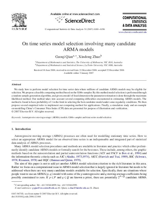Each score in the data represents the ratio of the current price to the one 12 months earlier. The data are plotted in Fig. 1a. It is well known that China’s economy has maintained a high speed of growth over the last 20 years or so. However, fluctuations in economy growths are also obvious. From Fig. 1a we see that China experienced two serious inflation periods in late 1980s and mid 1990s, respectively. The inflation rates during these two periods are almost as high as 30%. On the other hand, China experienced deflation in 1999 and 2002. To provide a valid model for analysing, the inflation rate is one of the major interests of statisticians and econometricians. A suitable class of time series models has to be identified first for such an analysis. Integrated ARMA models have been widely used for the time series data such as that of the CPI. By using the unit-root tests developed by Dickey and Fuller (1979) and Phillips and Perron (1988) we found that the first order difference of China’s CPI (denoted as DCPI, as shown in Fig. 1b) may be reasonably regarded as a stationary process. In fact, the augmented Dickey–Fuller test 6182 G. Qian, X. Zhao / Computational Statistics & Data Analysis 51 (2007) 6180 – 6196 a b China's CPI series between 12/1983 and 12/2003 The DCPI series 4 120 CPI DCPI 2 110 0 -2 100 -4 Dec 1983 c Dec 1991 Time in months Dec 1999 ACF plot with 95% confidence bands for DCPI Jan 1984 d Nov 1991 Time in months Sep 1999 PACF plot with 95% confidence bands for DCPI 1.0 0.4 ACF Partial ACF 0.6 0.2 -0.2 0.2 0.0 -0.2 0 5 10 Lag 15 20 0 5 10 Lag 15 20 Fig. 1. Plots for a preliminary analysis of the China’s CPI data. (a) China’s CPI series between 12/1983 and 12/2003. (b) The DCPI series. (c) ACF plot with 95% confidence bands for DCPI. (d) PACF plot with 95% confidence bands for DCPI. statistic is −2.06 with the p-value 0.55 for the CPI data; and, respectively, −8.62 and 0.01 for the DCPI data. We now apply Box–Jenkins preliminary model selection approach to determine a set of candidate ARMA models for the DCPI series. The sample ACF and PACF for the DCPI data are plotted in Figs. 1c and d. We see both the ACF and PACF plots are dominated by damped exponential and sine waves, which follow a typical pattern of those of the ARMA models. In addition, the ACF and PACF seem to be significant at some lags as high as up to 14 and 15, respectively. This suggests that an ARMA(p, q) model with p 15 and q 14 may be appropriate for the DCPI data. However, some of the AR and MA coefficients of ARMA(15, 14) may be more appropriately set to zero. Therefore, there would be in total 215+14 = 536, 870, 912 candidate ARMA models eligible for selection. Consequently, it is computationally infeasible to evaluate all the candidate models for finding the best model(s). This difficulty will be solved using the method developed in the following. 3. Model selection framework and criteria Consider a stationary and invertible ARMA(p, q) process {Yt }. Without losing generality assume the process {Yt } has mean 0. It is well known that {Yt } has the following representation: Yt = 1 Yt−1 + · · · + p Yt−p + εt + 1 εt−1 + · · · + q εt−q , (1) where {εt } is a sequence of white noise with mean 0 and variance 2 , and the polynomials 1 − 1 z − · · · − p zp and 1 + 1 z + · · · + q zq have no common factors and have no roots inside the unit circle |z| 1. G. Qian, X. Zhao / Computational Statistics & Data Analysis 51 (2007) 6180 – 6196 6183 Let Y1 , . . . , Yn be a sequence of observations from {Yt }. When the AR order p and MA order q are given, the unknown ARMA coefficients  = (1 , . . . , p ) and  = (1 , . . . , q ) and the innovation variance 2 may be estimated by the Gaussian maximum likelihood principle following Brockwell and Davis (2002, Sections 2.5.2 and 5.2). The Gaussian log-likelihood function for Y1 , . . . , Yn can be expressed in terms of the one-step prediction errors and their variances: log L(, , 2 ) = − n n n 1  (Yj − Ŷj )2 1 log rj −1 − 2 , log(22 ) − 2 2 rj −1 2 j =1 (2) j =1 where Ŷj = E(Yj |Y1 , . . . , Yj −1 , , ) is the one-step prediction of Yj ; E[(Yj − Ŷj )2 |Y1 , . . . , Yj −1 , , ] = 2 rj −1 is the conditional mean squared prediction error; and both Ŷj and rj −1 are functions of  and  but not 2 . Writing  2 2 S(, ) = nj=1 rj−1 −1 (Yj − Ŷj ) , one can then find that the Gaussian maximum likelihood estimate (MLE) of  is  ˆ 2 −1 −1 n ˆ ˆ of (, ) is the one that maximizes log L(, , 2 ) ˆ 2 =n−1 S(ˆ, )=n , ) j =1 r̂j −1 (Yj − Ŷ j ) . Further, the MLE (ˆ  or equivalently minimizes ℓ(, )=n log(n−1 S(, ))+ nj=1 log rj −1 where 2 is concentrated out. The minimization ˆ Such non-linear optimization of ℓ(, ) has to be done by a non-linear optimizer which numerically computes (ˆ, ). can sometimes be computationally very complicated and not stable (see computing manual of the arima function in R). On the other hand, the non-linear optimization involved can be much simplified if a so-called conditional loglikelihood approximation is used (see Bell and Hillmer, 1987;  MathSoft, 2000, Guide  to Statistics, vol. 2, 2p. 252). Namely, log L1 (, , 2 ) = −((n − m)/2) log(22 ) − ( 21 ) nj=m+1 log rj −1 − ( 21 2 ) nj=m+1 rj−1 −1 (Yj − Ŷj ) is used n −1 2 to replace log L(, ,  ), and ℓ1 (, ) = (n − m) log{(n − m) S1 (, )} + j =m+1 log rj −1 ≡ (n − m) log{(n −  n 2 m)−1 nj=m+1 rj−1 j =m+1 log rj −1 to replace ℓ(, ) in the optimization. This implies that the log−1 (Yj − Ŷj ) } + likelihood is conditional on the first m observations where mp at least. The resultant conditional MLE ˜ , ˜ and ˜ 2 usually have little difference from ˆ , ˆ and ˆ 2 . The question of what values of p and q should be used in an ARMA(p, q) model for {Y1 , . . . , Yn } can be answered by a model selection procedure. Knowing that the maximum possible values of p and q may be determined by some pre-model selection method such as that based on ACF and PACF, and that some components of the ARMA coefficients  and  may be taken 0, a more general model selection framework can be constructed as follows. Suppose a full ARMA model in which the AR order is P and the MA order is Q is given a priori for {Y1 , . . . , Yn }. We may denote the full model as ARMA(AF ; MF ) or simply (AF ; MF ) knowing that only ARMA models are considered. Here AF = (1, . . . , 1)1×P and MF = (1, . . . , 1)1×Q . Now a candidate model can be represented by ARMA(A; M) or (A; M) where A = (a1 , . . . , aP ) and M = (m1 , . . . , mQ ) are the indicator vectors defined as (1) ai = 1 if the model (A; M) includes the coefficient i and = 0 otherwise and (2) mj = 1 if (A; M) includes j and =0 otherwise. Note that a representation (A; M) only specifies which AR and MA coefficients are included in the model; thus the values of the included coefficients still need to be estimated. It is easy to see that given ARMA(AF ; MF ) there are in total 2P +Q candidate ARMA models. Now suppose a true model ARMA(Ao ; Mo ) (or ARMA(A; M)o ) exists for {Y1 , . . . , Yn } where Ao =(ao1 , . . . , aoP ), Mo =(mo1 , . . . , moQ ) and the true values of the coefficients i and j included in (A; M)o do not equal 0, whereas the true values of the other i and j equal 0. Then all the 2P +Q candidate models of the form (A; M) = (a1 , . . . , aP , m1 , . . . , mQ ) can be classified into two groups: A1 = {(A; M)(A; M)o , i.e. ai aoi and mj moj for all i, j }, A2 = {(A; M)(A; M)o , i.e. ai < aoi and/or mj < moj for some i, j }. It is easy to see that any model in A1 contains all non-zero ARMA coefficients of the true model, whereas any model in A2 misses at least one non-zero ARMA coefficient of the true model. Note that it may be reasonably assumed that the true model is unique. Then any candidate model in A1 shall be a correct model and provide a valid basis for statistical analysis. This, however, is not true for any model in A2 . On the other hand, a correct model in A1 may contain redundant coefficients that are not included in the true model. Therefore, with many candidate models available it is necessary to apply a model selection criterion to find the valid and simple models. 6184 G. Qian, X. Zhao / Computational Statistics & Data Analysis 51 (2007) 6180 – 6196 Many ARMA model selection criteria frequently used in practice actually have the following common form of a penalized log-likelihood: MSC(A; M) = −2 log L(ˆA , ˆ M , ˆ 2AM ) + C(A; M), (3) where log L(ˆA , ˆ M , ˆ 2AM ) is the maximum Gaussian log-likelihood for the model ARMA(A; M) evaluated at the MLE (ˆA , ˆ M , ˆ 2AM ), and C(A; M) > 0 measures the complexity of the model ARMA(A; M). For the commonly used criteria AIC, AICC, BIC and HQC, the term C(A; M) is specified, respectively, as follows: ⎛ ⎞ Q P   AIC : C(A; M) = 2 ⎝ mj + 1⎠ , ai + i=1 ⎛ AICC : C(A; M) = 2 ⎝ P  i=1 j =1 ai + Q  j =1 ⎞ mj + 1⎠ n/ ⎝n − ⎞ ⎛ Q P   mj + 1⎠ log n, BIC : C(A; M) = ⎝ ai + i=1 ⎛ P  i=1 ai − Q  j =1 ⎞ mj − 2 ⎠ , j =1 ⎞ ⎛ Q P   HQC : C(A; M) = 2 ⎝ mj + 1⎠ log log n. ai + i=1 j =1 If the conditional log-likelihood approximation is used in parameter estimation, the first term of MSC(A; M) should be accordingly replaced by −2 log L1 (˜A , ˜ M , ˜ 2AM ) and n in C(A; M) be replaced by n−m. This variant of MSC(A; M) reduces the amount of computation for model selection and usually has little effect on the final model selected. A model selection criterion based on MSC(A; M) will select as the best model—denoted as ARMA(A∗ ; M ∗ ) or ARMA(A; M)∗ —the one that has the smallest MSC(A; M) value over all candidate models. The implementation of such a criterion is straightforward in practice when the number of candidate models is not very large. An exhaustive search procedure will do it. A minor practical issue is that sometimes the parameter estimation of a candidate model cannot be accurately carried out using any non-linear optimizer due to various reasons such as that the model is too close to the boundary of those stationarity and invertiability conditions. If this is the case we may simply leave out this model because it is unlikely to be a good model for application. If this computing problem happens to most candidate models, it may suggest that modelling of the data by an ARMA process is not appropriate and a different class of time series model should be used. A major issue for applying the criterion MSC(A; M) is that it becomes computationally infeasible if the number of candidate models 2P +Q is too large. (This is true even when P + Q is moderately large.) Also model selection by MSC(A; M) becomes less discriminating when none of the candidate models have clear-cut small criterion values. We will be focusing on the latter two issues in the next section. The asymptotic performance of MSC(A; M) can be studied using the same approach as provided by Hannan (1980) where only the selection of the ARMA orders was considered. We believe that similar results as those of Hannan’s can also be obtained based on the model selection framework introduced here. That is, under regularity conditions, the first term of MSC(A; M) for any candidate model in A1 has a difference from −2 log L(ˆAo , ˆ Mo , ˆ 2Ao Mo ) that in absolute value is bounded from above by O(log log n) almost surely (with probability 1); and this difference in absolute value is bounded from below by O(n) almost surely for any model in A2 . It therefore implies that BIC is strongly consistent in that it will select the true model (A; M)o in A1 almost surely; and AIC, AICC and HQC select one of the models in A1 almost surely. However, we will not pursue a rigorous probabilistic proof for these results in this paper as it requires a dedicated work involving probability theory and large sample asymptotic study which would be difficult and also different from the focus of this paper. 4. Model selection based on random sampling We have already known that when 2P +Q is very large, it is computationally infeasible to evaluate all the 2P +Q candidate models for model selection. However, if we are able to take a random sample of a manageable size from the G. Qian, X. Zhao / Computational Statistics & Data Analysis 51 (2007) 6180 – 6196 6185 2P +Q candidate models and know that the best model having the minimum MSC(A; M) value is in this sample, we would have no computational difficulty to identify this best model from the sample. Let us define exp{−MSC(A; M)} , (A;M)∈A1 ∪A2 exp{−MSC(A; M)} PSC (A; M) =  where  > 0 is a tuning parameter. It is easy to see that PSC is a probability mass function defined on the set of MSC values of the 2P +Q candidate models for the given data {Y1 , . . . , Yn }. Equivalently, PSC (A; M) can be regarded as the probability mass function for a (P + Q)-dimensional discrete random vector (A; M) defined on A1 ∪ A2 = {0, 1}P +Q . Note that saying (A; M) is random here has different meaning from that in a Bayesian approach. We do not mean the format vector (A; M) of the ARMA model underlying the observations is a random realization from the model space on which some prior probability distribution is defined. Rather, we mean a candidate model represented by (A; M) is to be randomly sampled for evaluation from the model space on which the model selection criterion defines a function mathematically the same as a probability distribution function. By its definition PSC is maximal at the best model ARMA(A∗ ; M ∗ ). Also those ARMA candidate models having relatively small MSC values will have relatively large PSC probabilities. Thus, when generating a random sample from the distribution determined by PSC (A; M), models with relatively small MSC values are more likely to be generated and be generated earlier and more frequently than those models with relatively high MSC values. Hence, performing model selection based on the random sample generated would at least enable us to identify most of the models having small MSC values. If the sample generated is sufficiently large, the best model (A∗ ; M ∗ ) having the smallest MSC value would almost surely be identified and be selected with the highest frequency. Now consider the marginal distribution of an individual component of (A; M) which clearly is a Bernoulli distribution. It is expected that the probability of “success” (defined as this component indicator being equal to 1) in this marginal distribution is likely to be small if the corresponding component of (A; M) equals 0 at (A∗ ; M ∗ ), and to be large otherwise. This property should also be possessed by the sampling marginal distributions based on a random sample generated from PSC . The above discussion suggests three ways of performing model selection based on a random sample generated from PSC : 1. Estimate the best model by the one having the smallest MSC value in the sample. 2. Estimate the best model by the one appearing most frequently in the sample. 3. Estimate the best model by the one whose ARMA indicator components have large estimates of the probability of “success”. These three model selection procedures will be expounded after we demonstrate how a random sample from PSC can be generated in the following. 4.1. A Gibbs sampler for simulating PSC For convenience of presentation, denote (A; M)k as the kth indicator component of (A; M) and  (A; M)−k as the sub-vector (A; M) taken away (A; M)k . It is easy to see that the normalization constant D = (A;M)∈A1 ∪A2 exp{−MSC(A; M)} in the definition of PSC is difficult to evaluate when 2P +Q is very large. On the other hand, the conditional distribution of (A; M)k given (A; M)−k is Bernoulli and does not involve D. Specifically, for k = 1, . . . , P + Q, Pr{(A; M)k = 1|(A; M)−k } = Pr{(A; M)k = 1|(A; M)1 , . . . , (A; M)k−1 , (A; M)k+1 , . . . , (A; M)P +Q } exp{−MSC(A; M)}|(A;M)k =1 = and exp{−MSC(A; M)}|(A;M)k =1 + exp{−MSC(A; M)}|(A;M)k =0 Pr{(A; M)k = 0|(A; M)−k } = 1 − Pr{(A; M)k = 1|(A; M)−k }. Based on the conditional distributions Pr{(A; M)k |(A; M)−k } (k =1, . . . , P +Q) we can apply the Gibbs sampler (see, e.g. Casella and George, 1992) to generate a sequence of ARMA models. After ignoring an initial segment of models, 6186 G. Qian, X. Zhao / Computational Statistics & Data Analysis 51 (2007) 6180 – 6196 the sequence can be regarded approximately as a sample from PSC . The sampling algorithm is detailed below: (0) (0) 1. Arbitrarily take an initial value (A; M)(0) = ((A; M)1 , . . . , (A; M)P +Q ), e.g. (A; M)(0) = (1, . . . , 1) the full model ARMA(P , Q). 2. Given that (A; M)(1) , . . . , (A; M)(h−1) have been generated, do the following to generate (A; M)(h) for h = 1, . . . , H . • Repeat for k = P + Q, P + Q − 1, . . . , 2, 1. • Randomly generate a random number from the Bernoulli distribution having the probability of “success”  (h−1) (h−1) (h) (h) Pr (A; M)k = 1|(A; M)1 , . . . , (A; M)k−1 , (A; M)k+1 , . . . , (A; M)P +Q . (h) • Deliver the number generated to be (A; M)k —the kth component of (A; M)(h) . Some remarks for the above-described algorithm shall be made here. Firstly, using Gibbs sampler for model selection can be found in different contexts in literature. Madigan and York (1995) and George and McCulloch (1997) have used the Gibbs sampler for generating the posterior distribution of the variable indicators in Bayesian linear regression and graphic model selection. Qian (1999) and Qian and Field (2002) have used the Gibbs sampler for robust regression model selection and generalized linear regression model selection. Brooks et al. (2003) have used the Gibbs sampler in the context of the simulated annealing algorithm for autoregressive time series order selection. But so far we have not seen the use of the Gibbs sampler for ARMA model selection. On the other hand, there are methods other than the Gibbs sampler that can be used to generate samples from PSC . For example, it is possible to use the Metropolis-Hastings algorithm where the operational transitional distribution at each generation step is chosen to be the discrete uniform over a neighbourhood of the latest model generated. In fact, many algorithms belonging to the general approach of Markov chain Monte Carlo may be used here. However, the Gibbs sampler seems to be among the simplest ones to be implemented. Secondly, the sequence (A; M)(1) , . . . , (A; M)(H ) generated is actually a Markov chain as any other sample sequence generated by a Markov chain Monte Carlo method. Thus, the sequence usually takes a burn-in period to be in equilibrium. Determining when the sequence reaches equilibrium can be equivalently done by checking whether the corresponding sequence of the MSC values has reached equilibrium from some point on. An empirical method to check this is to plot a modified individual point control chart, or I-chart, for the series of the generated MSC sequence under inspection. Regarding MSC as a random variable with the probability distribution determined by PSC , it can be easily proved that Pr{MSC − min MSCb Var(MSC) + (E(MSC) − min MSC)2 }b−2 (4) for any b > 0. Using this result, we may set a lower control limit of the I-chart to be min MSC, the minimum of the MSC √ series. An upper control limit of the I-chart may be chosen to be min MSC + 10 s 2 (MSC) + (MSC − min MSC)2 where s 2 (MSC), MSC and min MSC are, respectively, the sample variance, the sample mean and the sample minimum of the second half of the MSC series. Then we know the MSC series is always above the lower control limit; also there would be less than 10% of the MSC series to be over the upper control limit when the series is in equilibrium and min MSC, s 2 (MSC), MSC and min MSC are consistent estimates. Therefore, if less than 10% of the MSC series are observed to be over the upper control limit we would say there is no significant statistical evidence that the MSC series has not reached equilibrium. The idea underlying the above I-chart is basically as follows: we first divide the MSC series into two halves that are assumed to come from two different distributions. The upper control limit is essentially estimated based on the second half of the series to which the above-mentioned “10%” rule applies. However, if the two halves have the same distribution, the “10%” rule shall also apply to the first half. Finally note that, since Var(MSC), E(MSC) and min MSC are unknown before going through all the candidate models, we are never 100% sure whether or not the generated MSC series has reached equilibrium. Thirdly, in our Gibbs sampler algorithm the order of updating (A; M)k is from P + Q to 1. Namely, given a (h−1) (h) generated ARMA(A; M)(h−1) model we first update (A; M)P +Q to get (A; M)P +Q , and so on, until finally we update (h−1) (h) (A; M)1 to get (A; M)1 . We chose this order with a belief that the best model is more likely to have lower AR and MA orders than the full model ARMA(P , Q). In principle, the order of update does not affect the model selection result. But in practice it is likely to affect how fast the generated models get close to the best model. G. Qian, X. Zhao / Computational Statistics & Data Analysis 51 (2007) 6180 – 6196 6187 Fourthly, a computing complication involved in the current algorithm is that sometimes the complementary model (h−1) (h−1) (h−1) (h) (h) , . . . , (A; M)k−1 , 1 − (A; M)k , (A; M)k+1 , . . . , (A; M)P +Q ) for the currently sampled one ((A; M)1 (h−1) (h−1) (h−1) (h) (h) ((A; M)1 , . . ., (A; M)k−1 , (A; M)k , (A; M)k+1 , . . . , (A; M)P +Q ) cannot be numerically accurately estimated (i.e. the numerical computation does not converge and breaks down) so that in effect the transitional probability  (h−1) (h−1) (h) (h) (5) Pr (A; M)k = 1|(A; M)1 , . . . , (A; M)k−1 , (A; M)k+1 , . . . , (A; M)P +Q = 1 or 0. If this is the case, the sequence of models generated may get trapped at a model having local minimum MSC value. To avoid this complication, we modify the definition of MSC(A; M) in which, when the complementary model with regard to the currently sampled model is practically not estimable, we define the MSC value of the complementary model to be the MSC value of the currently sampled model plus 3/. By this modification, the model sequence generated from PSC will have a e−3 ≈ 5% chance to get out of the trap mentioned above. But the best model having the smallest MSC value under the original definition will still have the smallest modified MSC value. Thus, the best model will still have the highest PSC probability after the modification. Further, those good candidate models that have relatively small MSC values are highly likely to be practically estimable. So relative frequencies of these models being generated from PSC would only be positively affected under the modification. Finally, the tuning parameter  > 0 is used to adjust the Gibbs sampling algorithm so that neither too many nor too few distinct models are generated. The number of distinct models generated is negatively correlated to . If  is small, the MSC sequence generated by the algorithm may be very slow to progress into the neighbourhood of the minimum MSC. If  is large, the MSC sequence generated may bypass the minimum MSC too often to ever reach it. From our experience, one should choose such a  that the number of distinct models in a sequence of H models generated is roughly 0.3H but not smaller than 0.05H . 4.2. Method 1: find the best model from the sample When a sample of models (A; M)(1) , . . . , (A; M)(H ) is generated by the Gibbs sampler, the associated MSC values are accordingly obtained. Therefore, it is straightforward to find the model that has the smallest MSC value in the sample. This model can be regarded as an estimate of the best model. The effectiveness of this procedure depends on how likely the sample of the models generated contains the best model (A∗ ; M ∗ ) and/or the true model (A; M)o . We consider a general situation where the asymptotic results as described by Hannan (1980) hold. Namely, we can reasonably assume that (C.1) For any model (A; M) in A1 , 0 < log L(ˆA , ˆ M , ˆ 2AM ) − log L(ˆAo , ˆ Mo , ˆ 2Ao Mo ) = O(log log n) a.s., where log L(ˆA , ˆ M , ˆ 2AM ) is the maximum log-likelihood of ARMA(A; M) and log L(ˆAo , ˆ Mo , ˆ 2Ao Mo ) is the maximum log-likelihood of the true model. Here and in the sequel “a.s.” means “almost surely” with respect to the probability space determined by the time series {Y1 , . . . , Yn , . . .}. (C.2) For any model (A; M) in A2 , 0 > log L(ˆA , ˆ M , ˆ 2AM ) − log L(ˆAo , ˆ Mo , ˆ 2Ao Mo ) = O(n) a.s. Then we have the following result for PSC (A; M). Proposition 1. Suppose C(A; M) = o(n) in the definition of MSC(A; M). Let Pr(·) be a probability with respect to the probability distribution PSC (A; M). Then under conditions (C.1) and (C.2) we have (R.1) Pr(A1 ) = {1 + (2do − 1)e−|O(n)| }−1 a.s. where do = (R.2) Pr(A1 )/ Pr(A2 ) = (2do − 1)−1 e|O(n)| a.s. P +Q i=1 (A; M)oi . 6188 G. Qian, X. Zhao / Computational Statistics & Data Analysis 51 (2007) 6180 – 6196 (R.3) In addition, if O(log n)|C(A; M)| O(n) and C(A; M) is an increasing function with respect to P +Q i=1 (A; M)i , then   −1 Pr((A; M)o ) = PSC ((A; M)o ) = 1 + 2P +Q−do − 1 n−|O(1)| Pr(A1 ) a.s. The proof of the proposition is straightforward knowing that there are 2P +Q−do models in A1 , 2P +Q−do (2do − 1) models in A2 , and PSC ((A; M)(1) )/PSC ((A; M)(2) ) = e|O(n)| a.s. under conditions (C.1) and (C.2) for (A; M)(1) ∈ A1 and (A; M)(2) ∈ A2 . Now suppose in the process of generating an independent random sample from PSC (A; M) it generates a model in A1 for the first time after it has generated T1 − 1 non-A1 models; and it generates the true model (A; M)o for the first time after it has generated To − 1 other models. Then both T1 and To follow the geometric distribution and according to Proposition 1:    −1 t1 t1 do −|O(n)| a.s., (6) Pr(T1 > t1 ) = [1 − Pr(A1 )] = 1 − 1 + (2 − 1)e  −1   Pr(To > to ) = [1 − Pr((A; M)o )]to = 1 − 1 + 2P +Q−do − 1 n−|O(1)| ×[1 + (2do − 1)e−|O(n)| ]−1 to a.s. (7) Using (6), (7), the inequality log(1 − a) − a for a > 0 and the Proposition 1, the 95th percentiles of T1 and To , denoted as T1,0.95 and To,0.95 , can be found to satisfy    (8) T1,0.95  Pr(A1 )−1 log 20 ≈ 3 1 + 2do − 1 e−|O(n)| a.s.,     To,0.95  Pr((A; M)o )−1 log 20 ≈ 3 1 + 2P +Q−do − 1 n−|O(1)| 1 + (2do − 1)e−|O(n)| a.s. (9) The model sequence generated by our Gibbs sampler algorithm is not an independent sample from PSC . Rather it is a reversible Markov chain (after the modification as specified after (5) in Section 4.1 is applied to the algorithm) and becomes ergodic with the stationary distribution PSC (or the modification) after a burn-in period. This follows that the models generated after the burn-in period can be used as an i.i.d. sample from PSC for most purposes (cf. Robert, 1998, p. 2). Therefore, it is reasonable to expect that properties (8) and (9) also hold asymptotically for the sequence of models generated by our Gibbs sampler algorithm after the burn-in period. The results (8) and (9) provide us with some asymptotic statements about how many models need to be generated after the burn-in period in order that an A1 model or the true model (A; M)o will be generated for the first time with an approximate probability of 0.95. The results also provide information on T1,0.95 /2P +Q and To,0.95 /2P +Q , which is about the efficiency of the random search procedure as compared with the exhaustive search procedure. We now propose an empirical rule prompted by (8), (9) and the remarks in Section 4.1 for determining how many models need to be generated in our random search procedure: (E.1) Suppose an initial sequence of H0 models has been generated; and from this point on it has been determined by the I-chart defined in Section 4.1 that the generated model sequence has reached equilibrium. To reduce the initialization effect of the Gibbs sampler, the first 5% of the H0 models may be ignored in constructing the initial sample. P +Q (E.2) Find the model (A; M)′0 that has the smallest MSC value in the initial sample. Find d0′ = i=1 (A; M)′0i and R ′ the range of the MSC values in the initial sample. ′ ′ ′ ′ ′ ′ (E.3) Calculate T1,0.95 = T1,0.95 [1 + (2P +Q−d0 − 1)R ′−1 ]. = 3[1 + (2d0 − 1)e−R ] and To,0.95 ′ (E.4) Further generate a sequence of To,0.95 models from PSC using the Gibbs sampler algorithm. Then find the model ∗ (A; M) that has the smallest MSC value on the combined initial and newly generated model sequences, and use this model as an estimate of the best model (A∗ ; M ∗ ). ′ ′ In generating the sample of H0 + To,0.95 models, we actually have generated (H0 + To,0.95 ) × (P + Q) ARMA models (h) knowing that in the Gibbs sampler each generated model (A; M) involves computing P + Q transitional ARMA G. Qian, X. Zhao / Computational Statistics & Data Analysis 51 (2007) 6180 – 6196 6189 ′ models. In order to make an efficient use of the computing output we may instead search all the (H0 + To,0.95 )(P + Q) models to find the one with the smallest MSC value and use it as the best model estimate. Clearly, the best model ′ estimate obtained in this way has the MSC value at least as small as that chosen from the H0 + To,0.95 models. Further, ∗ ∗ while the best model estimate is naturally an estimate of the best model (A ; M ), it can also be regarded as an estimate of the true model (A; M)o under the situation governed by conditions (C.1) and (C.2). To illustrate the above empirical rule, consider an example where P + Q = 16, d0′ = 6, R ′ = 10 and H0 = 100. It can ′ ′ be found that T1,0.95 ≈ 3, To,0.95 ≈ 310. So in total (100 + 310) × 16 = 6560 ARMA models need to be generated by the Gibbs sampler; and with approximate 95% probability we are sure that the best model among the total 216 = 65, 536 candidate models can be found from this sample of 6560 candidate models. ′ Finally, note that when P + Q is large and d0′ is relatively small, To,0.95 tends to be very large so that generating a ′ sample of size H0 + To,0.95 may still be computationally infeasible. In this case, we will provide a different procedure to be detailed in Section 4.4 to overcome the difficulty. 4.3. Method 2: find the most frequent model in the sample As the probability function PSC attains the highest at the best model (A; M)∗ , when we have generated a sample from PSC we can use the model that appears most frequently in the sample as an estimate of (A; M)∗ . As the size of the generated models becomes larger and larger, the most frequent model should converge to the best model (A; M)∗ with probability 1 in the limit. However, compared to the method in Section 4.2, this method involves more computations in finding the progressive frequencies of the generated models and is thus less preferred. This method may be useful when there are multiple models which all have close to the smallest MSC values. In this situation, the sample relative frequencies of these multiple models provide a measure of their relative significances. 4.4. Method 3: estimate marginal distributions of the candidate models Note that an ARMA candidate model can be represented by a (P + Q)-dimensional vector (A; M) in the latticework {0, 1}P +Q = A1 ∪ A2 . From the joint distribution PSC (A; M) it is easy to find the marginal distribution for each component of (A; M). Namely, for each i = 1, . . . , P + Q,   Pr((A; M)i = 1) = PSC (A; M) = D −1 exp{−MSC(A; M)}, (A;M)i =1 Pr((A; M)i = 0) =  (A;M)i =0 PSC (A; M) = D −1 (A;M)i =1  exp{−MSC(A; M)}. (A;M)i =0 Let o be the subset of 1, 2, . . . , P + Q that identifies those components of the true model (A; M)o whose values are 1, i.e. o = {i | i ∈ (1, . . . , P + Q); (A; M)oi = 1}. Under conditions (C.1) and (C.2) and from Proposition 1 it is not difficult to derive the following results: Proposition 2. Using the same conditions and notations as in Proposition 1, we have for any i ∈ o (R.4) Pr((A; M)i = 1)  Pr(A1 ) = [1 + (2do − 1)e−|O(n)| ]−1 a.s.; (R.5) Pr((A; M)i = 0)  Pr(A2 ) = (2do − 1)e−|O(n)| [1 + (2do − 1)e−|O(n)| ]−1 a.s.; (R.6) Pr((A; M)i = 1)/ Pr((A; M)i = 0)(2do − 1)−1 e|O(n)| a.s. Proposition 2 essentially says that the marginal distributions of (A; M) corresponding to those non-zero components of (A; M)o have their probabilities of “success” significantly larger than their respective probabilities of “failure”, provided that the sample size n is large enough. Moreover, this property is not affected by P + Q and accordingly not by whether the number of candidate models 2P +Q is too large or not. Therefore, for a sufficiently long sample of models generated from PSC —(A; M)(1) , . . . , (A; M)(H ) —we estimate the marginal probability of “success” for 6190 G. Qian, X. Zhao / Computational Statistics & Data Analysis 51 (2007) 6180 – 6196  (h)  each component of (A; M) by its sample proportion, i.e. Pr((A; M)i = 1) = H −1 H h=1 (A; M)i , i = 1, . . . , P + Q.  The standard error of Pr((A; M)i = 1) has an upper bound 0.5H −1/2 .  We then propose to ignore those components i of (A; M) where, say, Pr((A; M)i = 1) < 0.5, and use the other  components of (A; M) to form an estimate—denoted as (A; M)— of the true model (A; M)o or the best ARMA model (A; M)∗ for modelling {Y1 , . . . , Yn }, i.e.   (A; M) = {(A; M)i | i ∈ (1, . . . , P + Q); Pr((A; M)i = 1) 0.5}.  By Proposition 2 we know (A; M) will asymptotically at least include those ARMA coefficients indexed by o , i.e. identi fied by the true model (A; M)o . So (A; M) will at least be a correct model in A1 asymptotically. Following the argument of Robert (1998, p. 2) the preceding discussion can be extended to the situation where {(A; M)(1) , . . . , (A; M)(H ) } is only an ergodic and reversible Markov chain with the stationary distribution PSC (or the modification), i.e. a sequence generated by our Gibbs sampler algorithm after reaching equilibrium. An advantage of the method that is based on estimating the marginal distributions is that the model sample size H does not needs to be very large and is unlikely to depend on whether the number of candidate models 2P +Q is too large  or not. As a rule of thumb, H can be determined from a pre-specified desired standard error  for Pr((A; M)i = 1), −2  i.e. H = (2) . Of course, it is possible that (A; M) still has not removed all the redundant ARMA coefficients in  comparison to the true model (A; M)o . But it is highly likely that (A; M) is a correct model simpler than the full  model. Regarding (A; M) as a new full model, it is possible to generate another random sample of models and conduct  a second round of search which may return a better estimate of the best model than (A; M). The detail is to be given in Section 4.5. Finally, based on the generated Markov chain {(A; M)(1) , . . . , (A; M)(H ) } the marginal probability Pr((A; M)i = 1) may be more precisely estimated by the so-called Rao–Blackwellized estimate:  ((A; M)i = 1) = H −1 Pr H  h=1 (h) Pr((A; M)i = 1 | (A; M)−i ) H 1  exp{−MSC(A; M)}|(A;M)i =1,(A;M)−i =(A;M)(h) −i  = . exp{−MSC(A; M)}| H (h) (A;M)i ∈{0,1} (A;M) =(A;M) h=1 −i −i  However, the estimate Pr((A; M)i =1) involves more computation, and since we only use an estimate of Pr((A; M)i =1) for deciding whether it is greater than 0.5 or not, we do not suggest to use this Rao–Blackwellized estimate in our method. 4.5. A multi-step random search procedure In most situations, using one of the methods in Sections 4.2–4.4 should be enough for carrying out an effective random model selection procedure. But there may be situations where any of these methods by itself does not work effectively. This is quite likely to be true when either there are far too many candidate models for selection or no clear-cut best model can be identified with significant probability. If this is the case, we propose to use the following multi-step random search procedure, which is essentially a mixture of the methods in Sections 4.2–4.4, in the hope that it can identify at least some of the close-to-best models. (M.1) Generate a sequence of models from PSC until it is deemed to be in equilibrium. Then continue to generate H ′ models from PSC . The size H, instead of being determined by To,0.95 in (E.3) which could still be very large, −2 is determined by H = (2) .   (M.2) Form the model (A; M) as defined in Section 4.4. The model (A; M) may be modified to include additional (A; M) components provided by the model having the smallest MSC in the current sample. P +Q    (M.3) Regard (A; M) as a new full model and consider only the sub-models of (A; M). Denote d̃ = i=1 (A; M)i . There are now only 2d̃ candidate models constituting the set Ad for further model selection. G. Qian, X. Zhao / Computational Statistics & Data Analysis 51 (2007) 6180 – 6196 6191  (M.4) Define PSC (A; M) = exp{−MSC(A; M)}/ (A;M)∈Ad exp{−MSC(A; M)} for (A; M) ∈ Ad . Then generate a sample of models from PSC (A; M) and find the model having the smallest MSC value in the sample  as described in Section 4.2. This model, if has a smaller MSC value than (A; M), will be used as an estimated best model for modelling {Y1 , . . . , Yn }. Alternatively, we may use an exhaustive search procedure in this step if feasible. (M.5) If in the sample from PSC there are some models having very close to each other MSC values, then sampling relative frequencies of these models are calculated based on this sample. The sampling relative frequencies are used to evaluate the relative significances of the corresponding sampled models. Note that if d̃ in (M.3) is not very large, say d̃ 20, the whole procedure above is quite feasible computationally. If d̃ is still large, then steps (M.2)–(M.4) may be repeated based on the sample generated from PSC . This may help to eventually identify some models that are close to the overall best model. In general, the above multi-step procedure can be modified by using different mixtures of the methods in Sections 4.2–4.4. This, together with some exploratory analysis and subject information of the data, should provide a comprehensive solution to the ARMA model selection involving large number of candidate models. 5. Simulations and a revisit to China’s CPI data For simplicity of presentation, we use only BIC in implementing our proposed model selection procedure in this section. Implementation using the other criteria AIC, AICC and HQC is the same but may produce somewhat different finite sample results due to their respective different asymptotic properties. All the computations were performed using S-PLUS 6.2. Estimation of each given ARMA model was performed using the S-PLUS function arima.mle. In generating a sample of models from PSC the tuning parameter  was always chosen to be 0.8 in our computing. Also we will use a new notation for expressing an ARMA(A; M) model: A and M will be represented by the positions of their non-zero components. For example, ARMA(11000100; 01) is represented by ((1, 2, 6); (2)) and ARMA(8, 5) is represented by ((1, . . . , 8); (1, . . . , 5)). Example 1. We have generated a time series Yt of 500 observations, plotted in Fig. 2a, from the following stationary and invertible ARMA process Yt = 0.9Yt−1 − 0.8Yt−2 − 0.4Yt−5 + 0.2Yt−6 + εt − 0.4εt−2 + 0.5εt−3 , where the white noise variance 2 = 1. Therefore, the true model for Yt can be represented by (A; M)o = ((1, 2, 5, 6); (2, 3)). Now we pretend that this true model is unknown to us, and we proceed to finding an ARMA model that is deemed to have the smallest BIC value so can serve as an estimate of the true model. Suppose the full model is chosen to be ARMA(8, 8), i.e. (AF ; MF ) = (1, . . . , 1)1×16 , so that there are 216 = 65536 candidate models in total for selection. We apply the empirical rule (E.1)–(E.4) for model selection where we choose H0 = 100 at first. Namely, 100 segments of ARMA models, each of size 16, are generated from the Gibbs sampler initially. Rather than take the last model of each segment to form an initial sample of size 100, we use all the 1600 models as the initial sample. The I-chart of the initial sample, given in Fig. 2b, shows no significant evidence that the equilibrium has not been attained. Also it is found that (A; M)′0 = ((1, 2, 5, 6, 7); (3, 4, 6)), d0′ = 8 and R ′ = 7.16 thus ′ ′ T1,0.95 = 4 and To,0.95 = 132. Now we generate a further sequence of 132 × 16 = 2112 models following the initial sample. The best model (A; M)∗ that has the smallest BIC value among the models generated so far is found to be the same as (A, M)o ; is achieved at the 167 × 16 = 2672th model for the first time; and has the BIC value 1446.914 that is also the smallest one among all the 65,536 candidate models. Note that from Fig. 2b there seems to have a significant drop in the BIC values of the generated models from about the 2672th model. However, the I-chart cannot detect any violation of equilibrium from the upper control bound calculated based on the sample of the 3712 models generated so far. In order to seek more information about this simulation study, we have in total generated 600 × 16 = 9600 models including the initial sample. Denote the generated models as M1 , . . . , M9600 for convenience of presentation. Using the newly calculated upper control limit, we see from the I-chart that the model sequence has reached equilibrium more definitely from M3712 on, if not so from M1600 on. We find there are 49 different models among M1 –M9600 . The 10 best models in M1 –M9600 are listed in 6192 G. Qian, X. Zhao / Computational Statistics & Data Analysis 51 (2007) 6180 – 6196 a Time series plot 4 Y_t 2 0 -2 -4 -6 0 100 200 300 400 500 Time b I-chart for the generated BIC sequence 1490 Upper control limit 1461.475 for generations 1 to 1600 Upper control limit 1466.438 for generations 1 to 3712 Upper control limit 1457.675 for generations 1 to 9600 BIC 1480 1470 1460 1450 0 2000 4000 6000 8000 Generation Fig. 2. Plots for Example 1. (a) Time series plot. (b) I-chart for the generated BIC sequence. Table 1 The 10 best models found in Example 1, their BIC values, their ranks among all the candidate models, and their respective relative frequencies of appearances among M81 –M3712 (Rel. Freq1), M81 –M4800 (Rel. Freq2) and M81 –M9600 (Rel. Freq3) ARMA model BIC Rank Rel. Freq1 Rel. Freq2 Rel. Freq3 ((1, 2, 5, 6); (2, 3)) ((1, 2, 5, 6, 7); (2, 3)) ((1, 2, 5, 6); (2, 3, 8)) ((1, 2, 5, 6, 8); (2, 3)) ((1, 2, 4, 5, 7); (3, 7)) ((1, 2, 4, 5, 6); (2, 3)) ((1, 2, 5, 6, 7, 8); (2, 3)) ((1, 2, 5, 6); (1, 2, 3)) ((1, 2, 3, 5, 6); (2, 3)) ((1, 2, 5, 6); (2, 3, 6)) 1446.914 1450.185 1451.016 1451.184 1451.199 1452.006 1452.365 1452.767 1453.020 1453.062 1 4 6 8 9 13 15 21 24 27 0.219 0.030 0.009 0.010 0.000 0.002 0.001 0.004 0.002 0.004 0.348 0.043 0.010 0.016 0.000 0.002 0.004 0.010 0.005 0.003 0.441 0.048 0.013 0.012 0.157 0.005 0.007 0.005 0.004 0.003 Table 1, together with their BIC values and ranks with respect to BIC among all the 65,536 candidate models. We also list in Table 1 the frequencies of the above 10 best models generated in between M81 and M3712 , M81 and M4800 and M81 and M9600 , respectively. From these frequencies we see that the true and best model (A, M)o is always generated with the highest frequencies. However, sizeable variations can be found among the frequencies with respect to the sample size, suggesting that a much larger sample is required in order to achieve a consistent estimate of PSC . G. Qian, X. Zhao / Computational Statistics & Data Analysis 51 (2007) 6180 – 6196 6193 Table 2 Sample marginal probabilities of (A; M) based on the three model sequences M1601 –M3712 , M1601 –M4800 and M1601 –M9600 in Example 1 Sequence a1 a2 a3 a4 a5 a6 a7 a8 M1601 –M3712 M1601 –M4800 M1601 –M9600 1.000 1.000 1.000 1.000 1.000 1.000 0.030 0.030 0.016 0.053 0.040 0.240 1.000 1.000 1.000 0.864 0.910 0.756 0.550 0.398 0.409 0.038 0.045 0.036 Sequence m1 m2 m3 m4 m5 m6 m7 m8 M1601 –M3712 M1601 –M4800 M1601 –M9600 0.008 0.015 0.006 0.505 0.673 0.661 1.000 1.000 1.000 0.502 0.331 0.133 0.000 0.005 0.002 0.410 0.271 0.114 0.008 0.005 0.216 0.197 0.135 0.066 To see the performance of the method in Section 4.4, we list in Table 2 the sample marginal probabilities of each of the 16 (A; M) components, based on the models in between M1601 to M3712 , M1601 to M4800 and M1601 to M9600 , respectively. Again, there are sizable variations among the sample marginal probabilities with respect to the sample size. But the sample marginal probabilities corresponding to the non-zero components of (A; M)o , i.e. o = (1, 2, 5, 6, 10, 11), are all greater than 0.5; and those corresponding to the zero components of (A; M)o , i.e. co = (3, 4, 7, 8, 9, 12, 13, 14, 15, 16), are mostly much smaller than 0.5. Therefore, based on the sample marginal probabilities of (A; M) components, the true model (A; M)o is again selected as the best model. Finally, using the conditional likelihood approach, the best model (A; M)o is estimated to be Yt = 0.83Yt−1 − 0.78Yt−2 − 0.39Yt−5 + 0.17Yt−6 + εt − 0.50εt−2 + 0.46εt−3 with ˆ = 1.05 and the standard errors for the corresponding coefficients being 0.18, 0.08, 0.06, 0.10, 0.14 and 0.08. Example 2 (Example 1 continued). It can be found that two roots of the AR characteristic equation and one root of the MA characteristic equation are very close to the unit circle boundary for the ARMA model (A; M)o generating the data Yt in Example 1. This implies that the ACF for (A; M)o dies out quite slowly. Therefore, based on the sample ACF and PACF of Yt a much larger initial full model than ARMA(8, 8) may be found more appropriate. Here we choose ARMA(16, 16) to be used as the initial full model. This choice, which results in 232 candidate models, is not necessarily indisputable but simply used as an illustration to see the effects on model selection where there are too many candidate models. We now implement the multi-step procedure (M.1)–(M.5) described in Section 4.5. We first generate 100 segments of totally 100 × 32 = 3200 ARMA models using the Gibbs sampler, and have since found no significant evidence of not achieving the equilibrium from the I-chart (Fig. 3). Applying (E.2) and (E.3) of Section 4.2, it follows d0′ = 8, ′ R ′ = 46.2, T1,0.95 = 3 and To,0.95 = 1, 089, 433. Thus, we would need to generate 1, 089, 433 × 32 ARMA models if we were to apply (E.1)–(E.4) of Section 4.2, which is clearly infeasible. Therefore, we instead apply (M.1) by taking  = 0.025 and H = (2)−2 = 400; and generate a further 400 × 32 = 12, 800 ARMA models using the Gibbs sampler. The marginal probabilities of the 32 components of (A; M) are estimated from the lately generated 12,800 models with the results being given in Table 3. From those greater than 0.5 probability estimates we get a model  (A; M) = ((7, 8, 11, 13); (1, 2, 3, 9)) that serves as a first estimate of the best model. Further, it can be found that the model (A; M)′ = ((7, 11, 13); (1, 2, 3, 9)) has the smallest BIC value 1394.865 among all the 16,000 models generated and (A; M)′ appears first at the 4505th generation. Note that all the non-zero components of (A; M)′ have the corresponding marginal probability estimates greater than 0.60. Also note that (A; M)′ is very different from (A; M)o that has generated the data, but has a much smaller BIC value than (A; M)o . This is possibly due to the confounding effect of the random error involved in the data generation process and the state of near-boundary stationarity and invertibility for (A; M)o , so that the model selection criterion BIC is not able to identify the true model. But this is not the indication that the Gibbs sampler algorithm proposed in this paper cannot find the model having the smallest BIC value. Since the number of models that have been generated so far is much smaller than To,0.95 × 32 = 1, 089, 433 × 32, we suspect that there may be other models not yet being generated that have smaller BIC values than (A; M)′ . For this reason, we first check the BIC values of all the 27 − 1 = 127 sub-models of (A; M)′ and find that none of them have 6194 G. Qian, X. Zhao / Computational Statistics & Data Analysis 51 (2007) 6180 – 6196 I-chart for the generated BIC sequence 1520 Upper control limit 1465.626 for generations 1 to 3200 Upper control limit 1413.15 for generations 1 to 16000 1500 BIC 1480 1460 1440 1420 1400 0 5000 10000 15000 Generation Fig. 3. I-chart for equilibrium monitoring in Example 2. Table 3 Sample marginal probabilities of (A; M) obtained in Example 2 a1 a2 a3 a4 a5 a6 a7 a8 0.244 0.028 0.060 0.072 0.146 0.102 0.904 0.502 a9 a10 a11 a12 a13 a14 a15 a16 0.055 0.029 0.602 0.209 0.702 0.029 0.041 0.063 m1 m2 m3 m4 m5 m6 m7 m8 0.998 0.854 0.990 0.195 0.068 0.075 0.096 0.233 m9 m10 m11 m12 m13 m14 m15 m16 0.664 0.068 0.136 0.094 0.044 0.078 0.012 0.036  smaller BIC values. Secondly, we use ARMA(13, 9), which includes both (A; M) and (A; M)′ as sub-models, as the new full model and generate a sequence of 1000 × 22 = 22, 000 models following the empirical rule (E.1)–(E.4). From the sequence of models newly generated, we do not find any model having smaller BIC values than (A; M)′ either. In fact, those models having the smallest 5 BIC values in the new sequence are the same as those having the smallest 5 BIC values in the old sequence generated in (M.1). Hence, we can be reasonably confident that (A; M)′ is among those candidate ARMA models having the smallest BIC values. Example 3. We now reconsider the data on China’s CPI. In Section 2 we have seen that DCPI can be reasonably regarded as a stationary time series. Also we have known that an ARMA(15, 14) can be used as an initial full model. Here we first use the Gibbs sampler to generate an initial sequence of 100 × 29 = 2900 ARMA models; and by applying the empirical rule (E.1)–(E.3) we find that the initial sequence has reached equilibrium (see Fig. 4), (A; M)′0 = ′ ((1); (1, 11, 12)) with BIC 555.3013 and achieved at the 101th generation, and R ′ = 14.67. Also To,0.95 = 6, 860, 472 thus (E.4) cannot be feasibly applied. Instead, we apply the step (M.1) with  = 0.025 to generate a further sequence of 400 × 29 = 11, 600 models. The sample marginal probability estimates of (A; M) based on these 11,600 models and the total 14,500 models are listed in Table 4, respectively. From Table 4 we find those components with greater than G. Qian, X. Zhao / Computational Statistics & Data Analysis 51 (2007) 6180 – 6196 6195 I-chart for the generated BIC sequence for China s CPI data 660 Upper control limit 568.5614 for generations 1 to 2900 Upper control limit 570.5163 for generations 1 to 14500 640 BIC 620 600 580 560 0 2000 4000 6000 8000 10000 12000 14000 Generation Fig. 4. I-chart for equilibrium monitoring in Example 3. Table 4 Sample marginal probabilities of (A; M) obtained in Example 3 Sequence a1 a2 a3 a4 a5 a6 a7 a8 M1 –M14,500 M2901 –M14,500 1.000 1.000 0.042 0.028 0.026 0.028 0.014 0.013 0.014 0.015 0.042 0.045 0.018 0.020 0.016 0.018 Sequence a9 a10 a11 a12 a13 a14 a15 M1 –M14,500 M2901 –M14,500 0.019 0.013 0.099 0.108 0.015 0.017 0.045 0.044 0.031 0.033 0.027 0.028 0.021 0.015 Sequence m1 m2 m3 m4 m5 m6 m7 m8 M1 –M14,500 M2901 –M14,500 0.996 1.000 0.021 0.015 0.017 0.018 0.057 0.053 0.021 0.018 0.035 0.038 0.019 0.015 0.074 0.070 Sequence m9 m10 m11 m12 m13 m14 M1 –M14,500 M2901 –M14,500 0.092 0.088 0.060 0.060 0.712 0.700 0.998 1.000 0.018 0.020 0.018 0.018  0.5 probability estimates constitute the model (A; M) = ((1); (1, 11, 12)) = (A; M)′0 as per (M.2). Now we may use  (A; M) and actually we use ARMA(1, 12) as a new full model as per (M.3), and apply the step (M.4) with an exhaustive  search procedure. We find that none of the models generated in (M.4) has a smaller BIC value than (A; M)=(A; M)′0 = ((1); (1, 11, 12)). Therefore, we may reasonably use ((1), (1, 11, 12)) to estimate the best ARMA model for modelling the DCPI data. We list in Table 5 the 11 models that have the smallest 11 BIC values among the 14,500 models generated in (E.1) and (M.1), together with their frequencies of appearance in the sample. From this model selection procedure, it seems the most important autoregression dependence is at order 1 for the DCPI data; and the most important moving average dependance is at order 1, 11 and 12 indicating a 12-month period effect. Finally, the conditional likelihood estimate of the ARMA((1); (1, 11, 12)) model is Yt = 0.88Yt−1 + εt − 0.53εt−1 − 0.14εt−11 − 0.25εt−12 with ˆ = 0.77 and the standard errors of the estimated model coefficients being 0.049, 0.077, 0.073 and 0.068, respectively. 6196 G. Qian, X. Zhao / Computational Statistics & Data Analysis 51 (2007) 6180 – 6196 Table 5 The 11 best models obtained in Example 3 Model BIC Frequency ((1); (1, 11, 12)) ((1); (1, 12)) ((1); (1, 9, 11, 12)) ((1); (1, 8, 11, 12)) ((1); (1, 4, 11, 12)) ((1); (1, 10, 12)) ((1); (1, 10, 11, 12)) ((1); (1, 6, 12)) ((1, 10); (1, 11, 12)) ((1, 10); (1, 12)) ((1, 4); (1, 11, 12)) 555.3013 556.6439 557.7476 558.0147 558.4125 558.5644 559.3156 559.8965 559.9139 559.9608 559.9674 4970 1461 618 577 595 251 189 122 199 188 80 6. Conclusion In this paper we propose a Gibbs sampler-based computing method for ARMA model selection involving large number of candidate models. Such model selection is important in practice but seemingly is not well studied before. The essential idea underlying our method is that the best model can be found with high probability from a properly generated random sample of the candidate models. Implementing the method in practice, however, may encounter various complications; thus we have developed several empirical procedures to account for them. Through our investigations we have demonstrated that our method is computationally feasible, and is also effective and comprehensive. References Akaike, H., 1973. Information theory and an extension of the maximum likelihood principle. In: Petrov, B.N., Csáki, F. (Eds.), Proceedings of the Second International Symposium on Information Theory, Akadémia Kiadó, Budapest, pp. 267–281. Akaike, H., 1974. A new look at the statistical model identification. IEEE Trans. Automat Control AC-19, 716–723. Bell, W., Hillmer, S., 1987. Initializing the Kalman filter in the nonstationary case. ASA Proceedings of Business and Economic Statistics Section, pp. 693–697. Box, G.E.P., Jenkins, G.M., Reinsel, G.C., 1994. Time Series Analysis: Forecasting and Control. third ed. Prentice-Hall, New Jersey. Brockwell, P.J., Davis, R.A., 2002. Introduction to Time Series and Forecasting. second ed. Springer, New York. Brooks, S.P., Friel, N., King, R., 2003. Classical model selection via simulated annealing. J. Roy. Statist. Soc. Ser. B 65, 503–520. Casella, G., George, E.I., 1992. Explaining the Gibbs sampler. Amer. Statist. 46, 167–174. Dickey, D., Fuller, W.A., 1979. Distribution of the estimates for autogressive time series with a unit root. J. Amer. Statist. Assoc. 74, 427–431. George, E.I., McCulloch, R.E., 1997. Approaches for Bayesian variable selection. Statist. Sinica 7, 339–373. Hannan, E.J., 1980. The estimation of the order of an ARMA process. Ann. Statist. 8, 1071–1081. Hannan, E.J., Quinn, B.G., 1979. The determination of the order of an autoregression. J. Roy. Statist. Soc. Ser. B 41, 190–195. Hurvich, C.M., Tsai, C.L., 1989. Regression and time series model selection in small samples. Biometrika 76, 297–307. Madigan, D., York, J., 1995. Bayesian graphical models for discrete data. Internat. Statist. Rev. 63, 215–232. MathSoft, Inc., 2000. S-PLUS 6.0 Guide to Statistics, vol. 2. Data Analysis Division, MathSoft, Seattle, WA. Phillips, P., Perron, P., 1988. Testing for a unit root in time series regression. Biometrica 75, 335–346. Qian, G., 1999. Computations and analysis in robust regression model selection using stochastic complexity. Comput. Statist. 14, 293–314. Qian, G., Field, C., 2002. Using MCMC for logistic regression model selection involving large number of candidate models. In: Fang, K.T., Hickernell, F.J., Niederreiter, H. (Eds.), Selected Proceedings of the Fourth International Conference on Monte Carlo & Quasi–Monte Carlo Methods in Scientific Computing. Springer, Hong Kong, pp. 460–474. R Development Core Team, 2003. R: A Language and Environment for Statistical Computing. R Foundation for Statistical Computing, Vienna, Austria. URL: http://www.R-project.org . Rissanen, J., 1978. Modeling by shortest data description. Automatica 14, 465–471. Robert, C.P. (Ed.) 1998. Discretization and MCMC Convergence Assessment. Springer, New York. Schwarz, G., 1978. Estimating the dimension of a model. Ann. Statist. 6, 461–464.