Water Resour Manage (2014) 28:1327–1343 DOI 10.1007/s11269-014-0546-x Impact of Climate Change on the Hydrology of Upper Tiber River Basin Using Bias Corrected Regional Climate Model B. M. Fiseha & S. G. Setegn & A. M. Melesse & E. Volpi & A. Fiori Received: 11 October 2012 / Accepted: 2 February 2014 / Published online: 28 February 2014 # Springer Science+Business Media Dordrecht 2014 Abstract The use of regional climate model (RCM) outputs has been getting due attention in most European River basins because of the availability of large number of the models and modelling institutes in the continent; and the relative robustness the models to represent local climate. This paper presents the hydrological responses to climate change in the Upper Tiber River basin (Central Italy) using bias corrected daily regional climate model outputs. The hydrological analysis include both control (1961–1990) and future (2071–2100) climate scenarios. Three RCMs (RegCM, RCAO, and PROMES) that were forced by the same lateral boundary condition under A2 and B2 emission scenarios were used in this study. The projected climate variables from bias corrected models have shown that the precipitation and temperature tends to decrease and increase in summer season, respectively. The impact of climate change on the hydrology of the river basin was predicted using physically based Soil and Water Assessment Tool (SWAT). The SWAT model was first calibrated and validated using observed datasets at the sub-basin outlet. A total of six simulations were performed under each scenario and RCM combinations. The simulated result indicated that there is a significant annual and seasonal change in the hydrological water balance components. The annual water balance of the study area showed a decrease in surface runoff, aquifer recharge and total basin water yield under A2 scenario for RegCM and RCAO RCMs and an increase in PROMES RCM under B2 scenario. The overall hydrological behaviour of the basin indicated that there will be a reduction of water yield in the basin due to projected changes in temperature and precipitation. The changes in all other hydrological components are in agreement with the change in projected precipitation and temperature. B. M. Fiseha (*) : E. Volpi : A. Fiori Dipartimento di Scienze dell’Ingegneria Civile, Università di Roma Tre, Rome, Italy e-mail: fishbehulu@gmail.com B.. M.. Fiseha e-mail: fmuluneh@uniroma3.it B. M. Fiseha : S. G. Setegn : A. M. Melesse Department of Earth and Environment, Florida International University, Miami, FL 33199, USA 1328 B.M. Fiseha et al. Keywords RCM . Bias correction . Climate change . Hydrological modeling . SWAT . Tiber River basin 1 Introduction Global climate changes appear to affect most of the world’s water resources by altering the processes in the natural ecosystem. One of the most severe impacts will be the changes in regional water availability (Xu and Singh 2004). Such impacts have become a priority area of research and currently are intensely discussed by many researchers (e.g., Lettenmaier et al. 1999; Fowler et al. 2007). Studies indicated that climate change will pose two major water management challenges in Europe: increasing water stress mainly in southeastern part and increasing risk of floods in most part of the continent (Alcamo et al. 2007). The impacts on water resources are assessed considering various processes and storage behavior into account that include river flow and environmental requirement (Gul et al. 2010), water supply availability (Frederick and Major 1997; Bekele and Knapp 2010), regional water management (Cashman et al. 2010), flood frequency analysis (Prudhomme et al. 2002), regional groundwater assessment (Roosmalen et al. 2007; Woldeamlak et al. 2007; Loaiciga 2009) or groundwater recharge (Scibek and Allen 2006). Global Circulation Models (GCMs) have been developed to simulate the present climate and used to predict future climatic changes based on greenhouse gas and aerosol concentration as described in emission scenarios (IPCC 2000). In water resources impact assessment, there are varieties of GCM outputs at different spatial and temporal resolutions. However, they do not provide full representation of variables to the scale required by hydrological models. Therefore, downscaling of the large-scale variables to watershed scale variable, which is required by the hydrological models, has been a common approach (Xu et al. 2005; Fowler et al. 2007). Statistical and dynamical downscaling of the climate variables from GCM are the two known methods (Wilby and Wigley 1997). The statistical downscaling techniques involve developing quantitative relationships between large-scale atmospheric variables and local surface variables. The dynamical downscaling method involves the use of Regional Climate Models (RCMs) that are developed based on the same representations of atmospheric dynamical and physical processes as GCMs. As a result of their higher spatial domain (10–50 km), RCMs provide a better description of orographic effects, land-sea surface contrast and landsurface characteristics (Christensen and Christensen 2007). However, the RCMs are computationally demanding and susceptible to systematic model errors caused by imperfect conceptualization, discretization and spatial averaging within grid cells (Teutschbein and Seibert 2010). Therefore, bias correction of the RCM outputs for hydrologic impact assessment is recommended (Wood et al. 2004; Ines and Hansen 2006; Teutschbein and Seibert 2010). The use of RCM outputs has got due attention in most European River basins because of the availability of large number of models and modelling institutes in the continent. Among others, the Prediction of Regional scenarios and Uncertainties for Defining EuropeaN Climate change risks and Effects-PRUDENCE (Christensen et al. 2007), ENSEMBLE (van der Linden and Mitchell 2009) and the recently underway Coordinated Regional climate Downscaling Experiment-CORDEX (http://cordex.dmi.dk/joomla/) are the known ones under European Union (EU) funded integrated projects. Studies on the effect of climate change on water resources have been conducted by different researchers (e.g., Chavez-Jimenez et al. 2013; Zargar et al. 2014; Hanel et al. 2013). Various studies have been conducted by utilising these RCM outputs for hydrological analysis. Some of the examples are the studies of the effects of climate change on groundwater assessment Impact of Climate Change on the Hydrology of Upper Tiber River Basin 1329 (Roosmalen et al. 2007), runoff estimation (Rigon et al. 2007), flood risk assessment (Fowler and Wilby 2010), precipitation and potential evapotranspiration estimation (Baguis et al. 2010). Graham et al. (2007a) has used two bias correction methods (i.e. delta approach and scaling approach) to evaluate the impact of climate change on the hydrology of northern Europe using seven ensembles of RCMs and two GCM scenarios. The two methods gave similar mean results, but considerably different seasonal dynamics. Hence, one can deduce that the problem of stationarity remains unsolved as extreme conditions are not taken into account in this method. As a means to overcome such issues, Seguí et al. (2010) have used the quantilemapping method to evaluate the uncertainty related to the bias-corrections. However, in order to provide optimized climate scenarios for climate change impact assessment, Themeßl et al. (2010) have proposed merging of linear and nonlinear empirical-statistical techniques with bias correction methods and investigated their ability for reducing RCM error characteristics. They also found that quantile mapping shows the best performance, particularly at high quantiles, which is advantageous for applications related to extreme precipitation events. So far, comprehensive assessment of climate change projection with respect to hydrology is not available in Italy. However Coppola and Giorgi (2010), provides valuable information on precipitation and temperature characteristics of the country. They have shown that the use of RCMs is considered as suitable tools to simulate the climate of Italy much better than that of the GCMs. At regional scale, the precipitation and temperature characteristics of the Umbria region (central Italy) was studied by Todisco and Vergni (2008) and Vergni and Todisco (2011) with due emphasis on the extreme events and their impacts on crop production. The present work was necessitated to study the watershed scale impact of climate change on the major components of the upper Tiber River basin water budget using downscaled temperature and precipitation and the Soil and Water Assessment Tool (SWAT) model. The main objective of this study is to analyze the hydrological behavior of the sub-basin in the face of climate change using three RCMs under two emission scenarios. The flow characteristics at the basin outlet were explored on annual and seasonal basis. 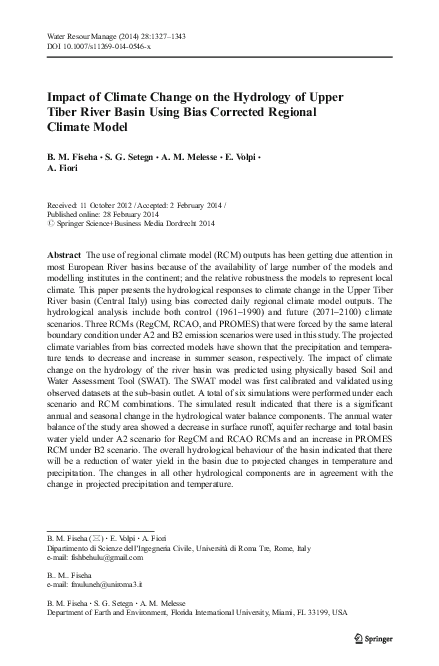2 Study Area Description The north–south elongated narrow Italian territory (between 36° and 41°N) is characterized by very pronounced, complex and fine-scale variability in topography, coastlines and vegetation cover. Tiber River basin is the largest river basin found in central Italy with different local effects. In this study, the upper part of the basin located between 42.6°–43.85°N and 11.8°– 12.9° E in the Umbria region of the main Tiber River basin was considered. It covers an area of 4145 km2 (nearly 20 % of the Tiber River basin) with elevation ranging from 145 to 1560 m above sea level (Fig. 1). The mountainous topography and the Italian Appennine in the eastern part of the sub-basin represent important physical boundaries that cause variability in precipitation and temperature. The climate of the area is characterized by Mediterranean climate with precipitation occurring mostly from autumn to spring seasons. The hydrology of the basin is highly influenced by the intense rainfall at the upstream part that causes frequent floods in the downstream areas (Calenda et al. 2000). In addition to the main Tiber River that originates near Montecoronaro, the basin is drained by three tributaries including: (i) the Chiascio and Topino rivers draining the upper part; (ii) the Paglia River from the right part; and (iii) the Velino and Aniene rivers draining the lower left part of the basin. Chiascio and Topino rivers cover larger area (>4000 km2) with the outlet at Ponte Nuovo station. The surface flow lag 1330 B.M. Fiseha et al. Fig. 1 Location and DEM of the Upper-Tiber River Basin time is assumed to be 18–22 h (Calenda et al. 2000). This sub-basin has also got relatively dense observation station in terms of precipitation and temperature as compared to the others. Therefore, this sub-basin is the main concern of the present study. The precipitation of the area is highly predominated by frontal processes coming from the Thyrrhenian Sea and orographic effect resulting from the high elevation ranges. The lithology of sub-basin is prevailed by calcareous and carbonaceous rocks, which characterize the basin with low permeability mainly on the upstream part. The land cover in the sub-basin is predominated by agricultural land (~40 %), forested areas (~ 50 %) and the remaining mixed land cover including urban land use areas account about 10 %. The forested area perhaps Impact of Climate Change on the Hydrology of Upper Tiber River Basin 1331 consists of deciduous forests, evergreen forest land, shrubs and rangelands distributed over the sub-basin. 3 Materials and Methods The study reported in this paper used regional climate model output for the assessment of future hydrologic regime in the selected sub-basin following three major steps. First, the hydrologic model is calibrated and validated using observed climate variable; second, the RCM outputs were selected from the available source and bias correction is applied at each gauging station based on the control period (1961–1990); and third, the bias corrected RCM outputs were used to force the calibrated and validated hydrologic model in order to understand the hydrologic behavior of the basin for the scenario period. For the hydrological analysis, the model is set to run for the period of 1961–1990 as a control period and 2071–2100 as a scenario period under the two emission scenarios of the three selected RCMs. The high and low flow behavior is then evaluated by constructing the flow duration curves (FDCs) on mean monthly and seasonal base. For such analysis, the FDC was classified into different segments following the subjective classification proposed by Yilmaz et al. (2008). The classification include: i) high-flow segment (0–20 % flow exceedance probability) characterizing watershed response to large precipitation events; ii) midsegment (20–70 % flow exceedance probability) representing flows controlled by moderate precipitation events coupled to medium-term base flow; and iii) a low flow-segment (70– 100 % exceedance probability) representing a catchment response dominated by long-term base flow during the extended dry periods. 3.1 Climate and Hydrology Data In this study, the historical precipitation, temperature (minimum and maximum) and flow data for the study area have been obtained from the hydrographic service of Umbria Region (IRSACNR). Based on the observed data in the period of 1961–1995, the mean annual rainfall is about 975 mm. The maximum monthly precipitation occurs in November (127 mm) and the minimum in July (44 mm). In the summer period, the average minimum and maximum temperature are 15.9 °C and 27.4 °C respectively; whereas in the winter period they are 2.3 °C and 8.9 °C respectively. The distribution of the selected weather and flow gauging stations are shown in Fig. 1. For calibration of the hydrologic model, daily flow data for the period of 1961–1970 at the sub-basin outlet was considered. The average daily discharge for this period was 47.93 m3 s−1 with a minimum value of 1.95 m3 s−1 and maximum value of 917 m3 s−1. Observed flow at three upstream gauging stations namely: Santa Lucia, Ponte Felcino and Petrignano di Assisi were used for validation purpose. 3.2 Description of the Hydrological Model In the present study, a physically based, semi distributed model, operating on daily time step called SWAT (Arnold et al. 1998) is used for simulation of watershed response in the study area. The model is capable of simulating various hydrological processes in different part of the world and intensely discussed in scientific literatures (Gassman et al. 2007). For rainfall-runoff simulation, the model divides the main basin under consideration into sub-basins connected through stream network that allows routing of flows to the downstream 1332 B.M. Fiseha et al. sections. The sub-basins are further subdivided into homogeneous Hydrological Response Units (HRUs), which is a lumped land area within a sub-basin comprised of unique land cover, soil, slope and management combinations. In each HRU, water balance is represented by several storage volumes: canopy storage, snow, soil profile (0–2 m), shallow aquifer (typically 2–20 m), and deep aquifer (≥20 m). The hydrologic cycle in the land phase as simulated by SWAT is based on the water balance equation: SW t ¼ SW o þ t  X i¼1 Rday −Qsurf −E a −W seep −Qgw  ð1Þ where SWt is the final soil water content (mm), SWo is the initial soil water content on day i (mm), t is the time (days), Rday is the amount of precipitation on day i (mm), Qsurf is the amount of surface runoff on day i (mm), Ea is the amount of evapotranspiration on day i (mm), wseep is the amount of water entering the vadose zone from the soil profile on day i (mm), and Qgw is the amount of return flow on day i (mm). The main inputs for SWAT model setup are the weather data (precipitation and temperature), Digital Elevation Model (DEM), landuse/landcover data. Observed precipitation and temperature dataset were obtained from the hydrographic service of Umbria Region. Basin characteristics such as slope gradient, slope length, stream network and stream characteristics (channel slope, length and width) were derived from the DEM using the automatic watershed delineation tool in the recent version of ArcSWAT. Land use/land cover data were obtained from the Medium Resolution Imaging Spectrometer (MERIS) public source. The soil datasets from Institute for Environment and Sustainability of the European commission Joint Research Center (JRC) were used as input to the model. The model setup was performed following four major steps: (i) watershed delineation and derivation of sub-basin characteristics (ii) hydrological response unit definition (iii) model run and parameter sensitivity analysis; and (iv) calibration and validation of the model including uncertainty analysis. Details on the input datasets, and model setup with the calibration and validation processes were explained in Fiseha et al. (2013). 3.3 Regional Climate Model Outputs In this paper, we have used dynamically downscaled air temperature and precipitation datasets for the central Italy archived in PRUDENCE project. The PRUDENCE was a project in the EU 5th Framework program for Energy, environment and sustainable development which was finished in 2004 (Christensen and Christensen 2007). It includes ensembles of ten RCMs with sets of simulations over 30-year length for control period of 1961–1990 and future period of 2071–2100 with forcing from the A2 and B2 emission scenarios (IPCC 2000). The A2 (medium-high) scenario describes a very heterogeneous world and B2 (medium-low) scenario describes a world in which the emphasis is on local solutions to economic, social and environmental sustainability. The set of scenario spans in the IPCC’s range with the A2 being close to the high end of the range (CO2 concentration of about 850 ppm by 2100) and B2 scenario lies towards the low end (CO2 Concentration of about 620 ppm by 2100). All the PRUDENCE RCMs experiments are limited to the European window at a grid spacing of about 50 km and are driven by different GCMs as their lateral boundary forcing fields (Christensen and Christensen 2007). The Hadley Center high resolution atmospheric model, HadAM3H Buonomo et al. (2007) is the central GCM delivering lateral boundary conditions Impact of Climate Change on the Hydrology of Upper Tiber River Basin 1333 to the RCMs used for the PRUDENCE standard ensemble (Jacob et al. 2007). This study used three regional climate models that were driven by HadAM3H for both A2 and B2 scenarios. The experimental set-up and brief description about the RCM models, participating institutes and GCM boundary forcing used in PRUDENCE are well explained in (Jacob et al. 2007; Christensen and Christensen 2007). The summary of models used in the present study is given in Table 1 3.4 Interfacing Between RCM and Hydrological Model The PRUDENCE-RCM outputs represent daily areal average values at the model resolution (~50 km) rather than the local values that make them not to be used directly in hydrological models. Moreover, the RCM outputs are reported to have inherent systematic biases due to their imperfect conceptualization, discretization and spatial averaging within grid cells (Graham et al. 2007a). Therefore, in order to use the RCM outputs in the SWAT model further correction was made on precipitation and temperature data. Due to the availability of numerous numbers of such RCMs a number of studies have been conducted in the past. Teutschbein and Seibert (2010), Teutschbein et al. (2011), and Teutschbein and Seibert (2012) provided a recent review on the use of RCMs for hydrological models. They recommend that a bias correction is necessary for using the outputs in any hydrological models as RCMs are susceptible to systematic model errors caused by imperfect conceptualization, discretization and spatial averaging within grid cells. These biases are typically due to the occurrence of too many wet days with low-intensity rain or incorrect estimation of extreme temperature in RCM simulations. Bias correction is also recommended by Wilby et al. (2006) and Wood et al. (2004) as a minimum requirement when using RCM outputs in hydrological impact studies. A simple bias correction method is used to prepare climate inputs to the model. This method was used in many studies (Lenderink et al. 2007; Roosmalen et al. 2007, 2010; Graham et al. 2007a; Teutschbein and Seibert 2010). The method is commonly applied to transfer the signal of climate change derived from a climate model simulation to an observed database. This study used the method following the work of Graham et al. (2007a) and et al. Lenderink et al. (2007) as they are termed as ‘scaling’ or ‘direct forcing’ approaches respectively. In this method, the changes derived for the control simulation of a particular climate model are applied to adjust scenario simulations from the same RCM. The observed Table 1 Selected regional climate model for hydrological impact assessment in the Upper Tiber River Basin Institute RCM (references) Resolution ITCP RegCM (Giorgi et al. 1993a, b) 50–70 km UCM PROMES (Arribas et al. 2003) 0.5° (~55 km) RCAO (Arribas et al. 2003) 0.44° (~50 km) SMHI GCM PRUDENCE acronyms Control (1961–1990) Scenario (2071–2100) HadAM3H A2 HadAM3H B2 Ref A2 B2 HadAM3H A2 Control HadAM3H B2 HadAM3H A2 HadAM3H B2 A2 B2 HCCTL A2 B2 ITCP International Center for Theoretical Physics, SMHI Swedish Meteorological and Hydrological Institute; UCM Universidad Complutense de Madrid 1334 B.M. Fiseha et al. precipitation at each station was compared with the nearest grid point of the RCM considering the grid points as a single station on the watershed. The correction procedures adopted in this study are explained in the following equations: For temperature: T corrected ði; jÞ ¼ T scen ði; jÞ þ ΔT ð jÞ; ΔT ð jÞ ¼ T obs ð jÞ−T ctrl ð jÞ; ð2Þ ð3Þ where: Tcorrected is the bias corrected temperature input for the hydrological model during the scenario simulation; Tscen is the simulated temperature in the scenario period; (i,j) is the ith day of jth month; ΔT(j) is the change in temperature between the observation and climate model during the reference period. T is the mean daily temperature for the month of j, which is calculated as the mean of all days in month j for all reference period (usually taken as 30 years). The indices scen and ctrl stand for the scenario period and control period (commonly taken as from 1960 to 1990 and 2070–2100), respectively. For precipitation: Pcorrected ði; jÞ ¼ Pobs ði; jÞ • ΔPð jÞ; ΔPð jÞ ¼ Pobs ð jÞ ð4Þ ð5Þ Pctrl ð jÞ where: Pcorrected is precipitation input for the hydrological scenario simulation; Pobs is the observed precipitation in the historical period at each station; (i,j) is the ith day of jth month; ΔP(j) is the change in precipitation calculated using as a ratio. Pð jÞ is the mean daily precipitation for the month of j, which is calculated as the mean of all days in month j for all reference period (usually taken as 30 years). The indices obs and ctrl stand for the observed and control period (1961–1990), respectively. In both cases, the mean monthly biases correction factors for each 30-years period of climate outputs for both scenarios (A2 and B2) were calculated and applied to daily simulations. Therefore a total of six simulations were performed using three RCMs and two emission scenarios. The simplified flow chart shown in Fig. 2, describes the general procedures followed in this paper. 4 Results and Discussions 4.1 Calibration and Validation Results of SWAT Model The behavior of the basin in terms of response to stream flow at the outlet were successfully evaluated by identifying the most sensitive parameters. Before applying the climate scenario into the model, calibration and validation was performed using observed flow at the basin outlet. Out of the twenty-six available hydrological parameters in the SWAT model, eighteen relevant parameters were evaluated and the top ten parameters were used following sensitivity analysis. The calibration was performed at the Impact of Climate Change on the Hydrology of Upper Tiber River Basin 1335 Fig. 2 A simple flow chart to use bias corrected RCM outputs in SWAT model basin outlet and the validation was done using independent dataset at the Ponte Nuovo station and three other upstream sub-basin outlets. All the performance indicators showed acceptable limits recommended by Moriasi et al. (2007). Results of sensitivity analysis and choice of parameters was given by Fiseha et al. (2013) in their previous work on the study area. Short summary of model calibration and validation results are shown in Table 2. The model performance during the calibration and validation period was shown in Figs. 3 and 4 respectively. 4.2 Bias Correction Results of Precipitation and Temperature Variables The monthly bias corrections between the observed and simulated variables during the control period for each RCM models were applied at each rainfall and temperature stations. The methods we used is the same for all stations, hence for clarity we presented here using only one station as shown in Table 3. We also note that since the RCM simulations during the control period are the same for both A2 and B2 scenarios, the correction applied is also the same with their corresponding RCMs. After applying the correction, the changes due to climate scenario are evaluated. Again we used the same site for presentation purpose and the results are shown in Table 4. 1336 B.M. Fiseha et al. Table 2 Performance of the model during the calibration and validation periods Station Period Analysis ENS PBIAS RMSE MAE R2 Ponte Nuovo 1960–1970 Calibration 0.85 −0.52 18.95 13.44 0.85 Ponte Nuovo 1971–1978 Validation 0.80 4.52 21.9 13.9 0.81 Santa Lucia 1991–1995 Validation 0.81 −5.57 4.49 5.67 0.81 Ponte Felcino Petrignano di Assisi 1991–1995 1991–1995 Validation Validation 0.68 0.50 −7.78 −20.88 11.74 4.79 7.39 2.95 0.71 0.55 ENS Nash and Sutcliffe efficiency, PBIAS the Percent bias, RMSE Root Mean Squared Error, MAE Mean Absolute Error, R2 coefficient of determination From Table 3, it can be inferred that the regional climate model from ITCP (RegCM) showed relatively larger bias as compared to the other two models for precipitation. In case of temperature, it also shows higher warming during summer season than the others. This indicates that the difference in model parameterization and discretization produces different climate characteristics, even though they use the same lateral boundary forcing from HadAM3H. Such differences were assessed in detail by (Jacob et al. 2007) and it can be considered as one source of uncertainty. The changes in each variable during the scenario and control period after the monthly correction is applied are shown in Table 4. The same analysis was applied to all other stations; however, we have shown here the result for station at Assisi. From Table 4, the three models showed maximum decrease in precipitation during the summer (JJA) season ranging from 35 to 65 %. The summer temperature however increases in all seasons and all models with temperature magnitude reaching as high as 6 °C on average. This result is also consistent with the work of Coppola and Giorgi (2010). 4.3 Hydrological Response to Climate Change The calibrated and validated SWAT model was then forced by the bias corrected RCM outputs at each stations. In order to evaluate the response of the sub-basin to the magnitude of the rainfall, monthly flow duration curves (FDC) under the three RCMs were used. The effects of the two future scenarios were evaluated by constructing FDCs for the annual and seasonal flows. Figure 5 shows the monthly flow duration curves at the Ponte Nuovo sub-basin outlet. From all the FDCs, the monthly stream flows showed an overall decrease for both scenarios. Fig. 3 Calibration results for monthly flow at Pone Nuovo (1963–1970) Impact of Climate Change on the Hydrology of Upper Tiber River Basin 1337 Fig. 4 Simulated versus observed flow during validation periods However, in case of B2 scenario, the PROMES model showed an increase in flow while others showed the decrease in monthly flows. This is due to the winter (DJF) and Spring (MAM-not shown) flows over prediction of the PROMES model as shown in the left column of B2 scenario and it is also consistent with the precipitation increase for the same scenario. During the summer (JJA) season, almost all RCMs showed a reduction in projected flow under both scenarios. The high-flow segment (i.e., 0–20 % exeedance probability) showed a sharp fall in slope of the FDCs for all RCMs that indicate a characteristic signature of the subbasin to produce quick response to the inputs. This is also due to the fact that the basin under study is dominated by soils with low infiltration capacity. Moreover, the steep slope of the midsegment and the flatter slope of the lower segment indicate that the sub-basin has slower Table 3 Bias correction factors used to modify the simulated climate variables for station at Assisi RCM Jan Feb Mar Apr May Jun Relative correction factor for precipitation CAO 0.96 1.11 0.85 0.92 1.01 1.26 Jul Aug Sep Oct Nov Dec 1.57 1.78 1.47 0.88 1.01 0.93 PROMES 1.87 1.84 1.25 1.28 1.14 1.48 0.75 1.19 1.40 1.08 1.58 1.32 RegCM 1.56 2.11 1.68 1.36 1.38 2.17 2.05 2.53 2.16 1.47 1.98 1.54 0.88 0.81 2.36 3.65 2.78 1.47 −0.31 −0.32 0.29 0.18 0.14 −0.62 0.33 0.61 1.77 1.80 0.53 −0.82 Absolute correction factor for temperature RCAO Tmax 1.39 Tmin 0.07 0.82 1.37 1.19 0.09 PROMES Tmax 4.32 4.06 5.99 7.79 7.78 4.74 7.62 8.92 8.07 5.69 3.77 Tmin 1.13 Tmax 3.99 1.63 3.06 2.37 2.60 2.60 0.93 1.82 2.44 3.79 3.61 1.96 −1.57 −0.57 0.92 3.49 2.73 1.36 0.49 3.64 5.36 5.11 3.94 Tmin 2.16 2.45 2.35 1.40 −1.80 −1.80 −0.93 0.76 2.09 2.21 1.58 RegCM 1.96 6.52 1338 B.M. Fiseha et al. Table 4 Seasonal changes in precipitation (%) and temperature (o C) Season RCAO A2 PROMES B2 A2 RegCM B2 A2 B2 Precipitation DJF 4 14 8 25 −8 −2 4 −3 8 0 11 JJA −65 −35 −37 −25 −26 −31 SON −20 6 −5 −4 −18 −15 MAM −3 Temperature Tmax Tmin 3.5 3.26 1.87 1.86 3.37 3.7 2.2 2.46 3.69 3.58 2.16 1.86 Tmax 3.23 1.63 4.14 2.89 3.67 2.02 Tmin 3.06 1.96 3.31 2.54 3.36 1.85 Tmax 6.79 5.07 6.83 6.13 5.4 3.82 Tmin 5.65 4.18 5.66 5.05 5.44 3.83 Tmax 4.45 2.99 4.27 3.77 4.7 2.91 Tmin 4.02 2.83 4.03 3.56 4.19 2.26 groundwater response. Except the PROMES_B2 scenario, the clear gap between the control and scenario period FDCs in the mid segments therefore indicate a decrease in groundwater volume of the sub-basin but not that much significant. However, it is worth to note that the land use and soil characteristics were assumed to be unchanged which may not be the case in the future. Hence, some uncertainties associated to such basin characteristics have to be considered for further usage. Fig. 5 Monthly flow duration curves for flow at the sub-basin outlet (Ponte Nuovo). The upper panels show the FDCs for the A2 scenario and the bottom panels show the one for B2 scenario Impact of Climate Change on the Hydrology of Upper Tiber River Basin 1339 In order to understand more about the future water resources availability a basin water balance analysis was performed on annual basis using the hydrological components as simulated by the SWAT model (Table 5). The result showed that there is a significant decrease in surface runoff, total aquifer recharge and the total water yield for all the RCMs under A2 scenario. The total water yield in SWAT model is the summation of the surface water flow, the water that enters the stream from soil profile as lateral flow contribution, and the water that returns to the stream from the shallow aquifer minus the total loss of water from the tributary channels as a transmission through the bed and finally reach the shallow aquifer as recharge. It was shown that a small change in precipitation adversely affect the amount of water yield from the basin. The B2 scenario also shows a decrease in the water balance components for all RCMs except the PROMES. The comparison between the mean annual flow under the different scenarios and the control period simulations indicated that the mean annual stream flow shows annual reduction ranging from 23 to 28 % for A2 scenario and 6 to 11 % for B2 scenario with the exception of PROMES model (Fig. 6). 4.4 Uncertainty Issues and Further Considerations In the present study, we have seen different SWAT simulation results from three RCMs forced by the same GCM lateral boundary conditions from HadAM3H. Despite all the progressive uses and their added values to reproduce the forcing variables, various uncertainties still exists in using RCMs for hydrological impact assessment that require further considerations. The major sources of these uncertainties are explained in other research papers as a ‘cascaded’ form (Viner 2003; Giorgi 2005) which are inter-dependent, but not necessarily additive or multiplicative (New and Hulme 2000). While moving from GCM outputs to basin scale hydrological impact assessment as a top-down approach, the ‘cascaded uncertainty’ can be grouped into four (Xu et al. 2005; Praskievicz and Chang 2009). The first is due to the choice of GCMs (i.e. uncertainty due to climate scenarios). For example, in our case we have used the A2 and B2 emission scenarios which were resulted in different prediction of the hydrological component. The second is associated with the choice of the deriving GCM which is generally claimed as Table 5 Comparison of mean annual water balance for the control and scenario periods Hydrologic components Control (1961–1990) RegCM A2 RCAO B2 A2 PROMES B2 A2 B2 Precipitation 953 860 918 838 924 900 1099 Surface Runoff 137 97 110 79 101 105 158 Lateral flow 74 67 73 69 78 68 91 Shallow groundwater flow 149 101 137 115 160 105 220 Groundwater re-evaporation 97 112 107 113 107 115 113 Deep aquifer recharge Total aquifer recharge 27 275 25 247 28 280 26 260 30 305 25 252 38 375 Total water yield 356 262 317 259 335 274 464 Percolation out of soil 270 244 277 257 303 249 371 Evapotranspiration 472 451 456 433 442 478 479 Transmission losses 4 4 4 4 4 3 5 (All units are in mm) 1340 B.M. Fiseha et al. Fig. 6 Average annual change in river flow at Ponte Nuovo under A2 and B2 scenario the largest sources of uncertainty by many authors (Wilby et al. 2006; Fowler et al. 2007; Graham et al. 2007b; Prudhomme and Davies 2009). In the present study, only single GCM was used to force the three selected RCMs; therefore it is impossible to justify the range of uncertainty under this source. The third source of uncertainty is associated to the transfer of large-scale climatology to regional-scale climatology appropriate for hydrological impact assessment, which is commonly called as downscaling. In the present study, further bias correction is applied to dynamically downscale RCM models. We found different results which are susceptible to one of these sources of biases. The fourth is related to the parameters and structures of hydrological models used for impact assessment. Finally, the uncertainty due to input variables can also affect final result. Therefore, care needs to be taken while interpreting the simulated results for further usage in impact assessment. Quantitative determination of all the uncertainties explained above is the remaining research topic in climate change and impact assessment. However, few studies have evaluated the propagation of one uncertainty to the next until it reaches the final hydrologic impact study (Graham et al. 2007a, b; Prudhomme and Davies 2009) in the top-down approach for impact study. Beside all the uncertainties mentioned above, it is worth to note that the selection of emission scenarios based on the prescribed story lines have their own limitations, as there is no exact rule to predict the global socio-economic systems in the future. For example in the case of Upper Tiber Basin, we have seen completely different results between A2 and B2 scenarios but difficult to decide which one has correctly predicted the impact. 5 Conclusion This study presents the expected changes in precipitation and air temperature for the Upper Tiber River basin by the end of this century (2071–2100) using the three different regional climate models from the PRUDENCE project. A simple bias correction method of precipitation and temperature was applied to the dynamically downscaled RCMs. The correction is applied to stations nearby to each grid cells. Observed data from twelve rainfall stations and four temperature stations over an area of 4100 km2 were used. From the bias corrected results it can be inferred that the decrease in precipitation can reach up to 35 % and temperature changes reaches to 6 °C during dry summer (JJA). The Soil and Water Assessment Tool was successfully calibrated and validated based on observed flow and weather variables. Except the PROMES model under B2 emission scenario, all RCMs have shown significant reduction in stream flow at the sub-basin outlet. The sub- Impact of Climate Change on the Hydrology of Upper Tiber River Basin 1341 basin water balance has also resulted in significant reduction of surface runoff, aquifer recharge and total water yield. This is mainly due to the reduction in precipitation over the entire basin. This study mainly focused on the use of RCM output to evaluate the possible future climate impact under two different scenarios. The limitation of this study is that the three RCMs were derived from a single GCM. According to IPCC reports high uncertainty is expected in climate change impact studies if the simulation results of a single GCM output are relied upon. Acknowledgments This research work is partially funded by PRIN 2010–2011 (2010JHF437). The historical weather and flow data were collected from Hydrographic Service of Umbria Region. The authors are also grateful for the European Union PRUDENCE project for provision of dynamically downscaled RCM datasets free of charge. References Alcamo J, Moreno JM, Nováky B, Bindi M, Corobov R, Devoy RJN, Giannakopoulos C, Martin E, Olesen JE, Shvidenko A (2007) In: Parry ML, Canziani OF, Palutikof JP, van der Linden PJ, Hanson CE (eds) Europe: Ipcc Ar4. Climate Change 2007: Impacts, adaptation and vulnerability. Contribution of Working Group II to the Fourth Assessment Report of the Intergovernmental Panel on Climate Change. Cambridge University Press, Cambridge, pp 541–580 Arnold JG, Srinivasan R, Muttiah RS, Williams JR (1998) Large area hydrologic modeling and assessment—part 1: model development. J Am Water Resour Assoc 34(1):73–89 Arribas AA, Gallardo CG, Gaertner MG, Castro MC (2003) Sensitivity of the Iberian peninsula climate to a land degradation. Clim Dyn 20(5):477–489 Baguis P, Roulin E, Willems P, Ntegeka V (2010) Climate change scenarios for precipitation and potential evapotranspiration over central Belgium. Theor Appl Climatol 99(3–4):273–286 Bekele EG, Knapp HV (2010) Watershed modeling to assessing impacts of potential climate change on water supply availability. Water Resour Manag 24(13):3299–3320 Buonomo E, Jones R, Huntingford C, Hannaford J (2007) On the robustness of changes in extreme precipitation over Europe from two high resolution climate change simulations. Q J R Meteorol Soc 133(622):65–81 Calenda G, Casaioli M, Cosentino C, Mantovani R, Speranza A (2000) Flood forecasting in the Tiber catchment area: a methodological analysis. Ann Geofis 43(5):869–888 Cashman A, Nurse LA, John C (2010) Climate change in the Caribbean: the water management implications. J Environ Dev 19(1):42–67 Chavez-Jimenez A, Lama B, Garrote L, Martin-Carrasco F, Sordo-Ward A, Mediero L (2013) Characterisation of the sensitivity of water resources systems to climate change. Water Resour Manag 27(12):4237–4258 Christensen JH, Christensen OB (2007) A summary of the prudence model projections of changes in European climate by the end of this century. Clim Chang 81:7–30 Christensen JH, Carter TR, Rummukainen M, Amanatidis G (2007) Evaluating the performance and utility of regional climate models: the prudence project. Clim Chang 81:1–6 Coppola E, Giorgi F (2010) An assessment of temperature and precipitation change projections over Italy from recent global and regional climate model simulations. Int J Climatol 30(1):11–32 Fiseha BM, Setegn SG, Melesse AM, Volpi E, Fiori A (2013) Hydrological analysis of the Upper Tiber River Basin, Central Italy: a watershed modelling approach. Hydrol Process 27:2339–2351. doi:10.1002/hyp.9234 Fowler HJ and Wilby RL (2010). Detecting changes in seasonal precipitation extremes using regional climate model projections: implications for managing fluvial flood risk. Water Resour Res 46(W03525) Fowler HJ, Blenkinsop S, Tebaldi C (2007) Linking climate change modelling to impacts studies: recent advances in downscaling techniques for hydrological modelling. Int J Climatol 27(12):1547–1578 Frederick KD, Major DC (1997) Climate change and water resources. Climate Change 37:7–23 Gassman PW, Reyes MR, Green CH, Arnold JG (2007) The soil and water assessment tool: historical development, applications, and future research directions. Trans ASABE 50(4):1211–1250 Giorgi F (2005) Climate change prediction. Clim Chang 73(3):239–265 Giorgi F, Marinucci MR and Bates GT (1993a) Development of a second-generation regional climate model (Regcm2). Part I: Boundary-layer and radiative transfer processes. Mon Weather Rev 21: 2794–2813 1342 B.M. Fiseha et al. Giorgi F, Marinucci MR and Bates GT (1993b) Development of a second-generation regional climate model (Regcm2). Part II: Convective processes and assimilation of lateral boundary conditions. Mon Weather Rev 121:2814–2832 Graham LP, Andreasson J, Carlsson B (2007a) Assessing climate change impacts on hydrology from an ensemble of regional climate models, model scales and linking methods—a case study on the lule river basin. Clim Chang 81:293–307 Graham LP, Hagemann S, Jaun S, Beniston M (2007b) On interpreting hydrological change from regional climate models. Clim Chang 81:97–122 Gul GO, Rosbjerg D, Gul A, Ondracek M, Dikgola K (2010) Assessing climate change impacts on river flows and environmental flow requirements at catchment scale. Ecohydrology 3(1):28–40 Hanel M, Mrkvičková M, Máca P, Vizina A, Pech P (2013) Evaluation of simple statistical downscaling methods for monthly regional climate model simulations with respect to the estimated changes in runoff in the Czech Republic. Water Resour Manag 27(15):5261–5279 Ines AVM, Hansen JW (2006) Bias correction of daily GCM rainfall for crop simulation studies. Agric For Meteorol 138(1–4):44–53 IPCC (2000) Special Report on Emission Scenarios (Sres): A Special Report of Working Group Ii of the Intergovernmental Pannel on Climate Change. Cambridge University Press, Cambridge Jacob D, Bärring L, Christensen OB et al (2007) An inter-comparison of regional climate models for Europe: design of the experiments and model performance. Climate. Clim Chang 81:31–52 Lenderink G, Buishand A, Van Deursen W (2007) Estimates of future discharges of the river Rhine using two scenario methodologies: direct versus delta approach. Hydrol Earth Syst Sci 11(3):1145–1159 Lettenmaier DP, Wood AW, Palmer RN, Wood EF, Stakhiv EZ (1999) Water resources implications of globalwarming: A U.S. Regional perspective. Clim Chang 43:537–579 Loaiciga HA (2009) Long-term climatic change and sustainable ground water resources management. Environ Res Lett 4(3):11 Moriasi DN, Arnold JG, Van Liew MW, Bingner RL, Harmel RD, Veith TL (2007) Model evaluation guidelines for systematic quantification of accuracy in watershed simulations. Trans ASABE 50(3):885–900 New M and Hulme M (2000). Representing uncertainties in climate change scenarios: a Monte Carlo approach. Integr Assess 1 Praskievicz S, Chang HJ (2009) A review of hydrological modelling of basin-scale climate change and urban development impacts. Prog Phys Geogr 33(5):650–671 Prudhomme C, Davies RJ (2009) Assessing uncertainties in climate change impact analyses on the river flow regimes in the UK. Part 1: baseline climate. Clim Chang 93:177–195 Prudhomme C, Reynard N, Crooks S (2002) Downscaling of global climate models for flood frequency analysis: where are we now? Hydrol Process 16(6):1137–1150 Rigon R, Bellin A, Forlin AL, Fowler HJ, Blenkinsop S (2007). Testing of climate change scenarios on a casestudy catchment using different methodologies. AquaTerra Project Deliverable No: H1.9 Roosmalen VL, Christensen BSB, Sonnenborg TO (2007) Regional differences in climate change impacts on groundwater and stream discharge in Denmark. Vadose Zone J 6(3):554–571 Roosmalen VL, Christensen JH, Butts MB, Jensen KH, Refsgaard JC (2010) An intercomparison of Regional climate model data for hydrological impact studies in Denmark. J Hydrol 380(3–4):406–419 Scibek J, Allen DM (2006). Modeled impacts of predicted climate change on recharge and groundwater levels. Water Resour Res 42(11) Seguí PQ, Ribes A, Martin E, Habets FA, Boé J (2010). Comparison of three downscaling methods in simulating the impact of climate change on the hydrology of Mediterranean basins. J Hydrol 383 Teutschbein CA, Seibert J (2010) Regional climate models for hydrological impact studies at the catchment scale: a review of recent modeling strategies. Geogr Compass 4(7):834–860 Teutschbein C, Seibert J (2012). Bias correction of regional climate model simulations for hydrological climatechange impact studies: review and evaluation of different methods. J Hydrol (456–457): 12–29 Teutschbein C, Wetterhall F, Seibert J (2011) Evaluation of different downscaling techniques for hydrological climate-change impact studies at the catchment scale. Climate Dynamics: 1–19 Themeßl MJ, Gobiet A, Leuprecht A (2010) Empirical-statistical downscaling and error correction of daily precipitation from regional climate models. Int J Climatol 31(10):1530–1544 Todisco F, Vergni (2008) Climatic changes in central Italy and their potential effects on corn water consumption. Agric For Meteorol 148(1):1–11 van der Linden P, Mitchell JFB (2009) Ensembles: climate change and its impacts: summary of research and results from the ensembles project. Met Office Hadley Centre, Exeter, 160pp Vergni L, Todisco F (2011) Spatio-temporal variability of precipitation, temperature and agricultural drought indices in central Italy. Agric For Meteorol 151(3):301–313 Impact of Climate Change on the Hydrology of Upper Tiber River Basin 1343 Viner D (2003) A qualitative assessment of the sources of uncertainty in climate change impacts assessment studies. Climatic change: implications for the hydrological cycle and for water management. Springer Neth 10:139–149 Wilby RL, Wigley TML (1997) Downscaling general circulation model output: a review of methods and limitations. Prog Phys Geogr 21(4):530–548 Wilby RL, Whitehead PG, Wade AJ, Butterfield D, Davis RJ, Watts G (2006) Integrated modelling of climate change impacts on water resources and quality in lowland catchment: River Kennet, UK. J Hydrol 330:204–220 Woldeamlak ST, Batelaan O, De Smedt F (2007) Effects of climate change on the groundwater system in the Grote-Nete catchment, Belgium. Hydrogeol J 15:891–901 Wood AW, Leung LR, Sridhar V, Lettenmaier DP (2004) Hydrologic implications of dynamical and statistical approaches to downscaling climate model outputs. Clim Chang 62(1):189–216 Xu CY, Singh VP (2004) Review on regional water resources assessment models under stationary and changing climate. Water Resour Manag 18(6):591–612 Xu CY, Widen E, Halldin S (2005) Modelling hydrological consequences of climate change—progress and challenges. Adv Atmos Sci 22(6):789–797 Yilmaz KK, Gupta HV, Wagener T (2008) A process-based diagnostic approach to model evaluation: application to the Nws distributed hydrologic model. Water Resour Res 44(W09417) doi:10.1029/2007WR006716 Zargar A, Sadiq R, Khan FI (2014) Uncertainty-driven characterization of climate change effects on drought frequency using enhanced SPI. Water Resour Manag 28(1):15–40