RoboSoccer: Autonomous Robots in a Complex Environment Pieter P. Jonker, Jurjen Caarls, Wouter J. Bokhove, Werner Altewischer, Ian T. Young* Pattern Recognition Group, Faculty of Applied Sciences, Lorentzweg 1, Delft University of Technology, NL-2628 CJ Delft, The Netherlands ABSTRACT We are participating in the international competition to develop robots that can play football (or soccer as it is known in the US and Canada). The competition consists of several leagues each of which examines a different technology but shares the common goal of advancing the skills of autonomous robots, robots that function without a central hierarchical command structure. The Dutch team, Clockwork Orange, involves several universities and the contribution of our group at the TU Delft is in the domain of robot vision and motion. In this paper we will describe the background to the project, the characteristics of the robots in our league, our approach to various vision tasks, their implementation in computer architectures, and the results of our efforts. Keywords: robots, soccer, computer vision, color segmentation and classification, Hough transforms, camera calibration, analysis of robot performance 1 INTRODUCTION th Since at least the 16 century writers and artists have described machines that could serve man by relieving him of tedious work and replacing him in dangerous environments. Coupled with each of these visions of the future has been the fear that our creations could come to function outside of our control and themselves become dangerous. Perhaps the oldest legend is that of the “Golem” who was constructed from clay by Rabbi Löw in Prague in 1580 to protect the community. In the legend the Golem becomes a danger to the community. The word “robot” stems from the play “R.U.R.” written in 1920 by the Czech Karel Capek. “R.U.R.” stands for “Rossum’s Universal Robots” and the word robot comes from the Czech word “robota”, work. The concept of the robot was popularized in the 1950’s with a series of science fiction books and films such as Isaac Asimov’s novels emphasizing the computational (and moral) aspects in the “positronic brain” and the “Three Laws of Robotics”, the movie “Forbidden Planet, the “Star Wars” heroes/comics C3PO and R2D2, the “Terminator”, and “Blade Runner.” All of these examples would be irrelevant to modern research in robot vision, autonomous systems, and the latest incarnation of artificial intelligence were it not for the fact that these robots displayed independent behavior that could be achieved through sensors, actuators, and algorithmic analyses. The most timely example of this transfer from science fiction to technological reality has been the recent work at Boeing to develop robotic attack fighters, the Boeing X-45 project.1 At the forefront of university-led research into robotics, one of the most enchanting and inspiring is the RoboCup competition ( http://www.robocup.org/ ) where the goal is to develop robots that can play football or, as it is known in the US and Canada, soccer. 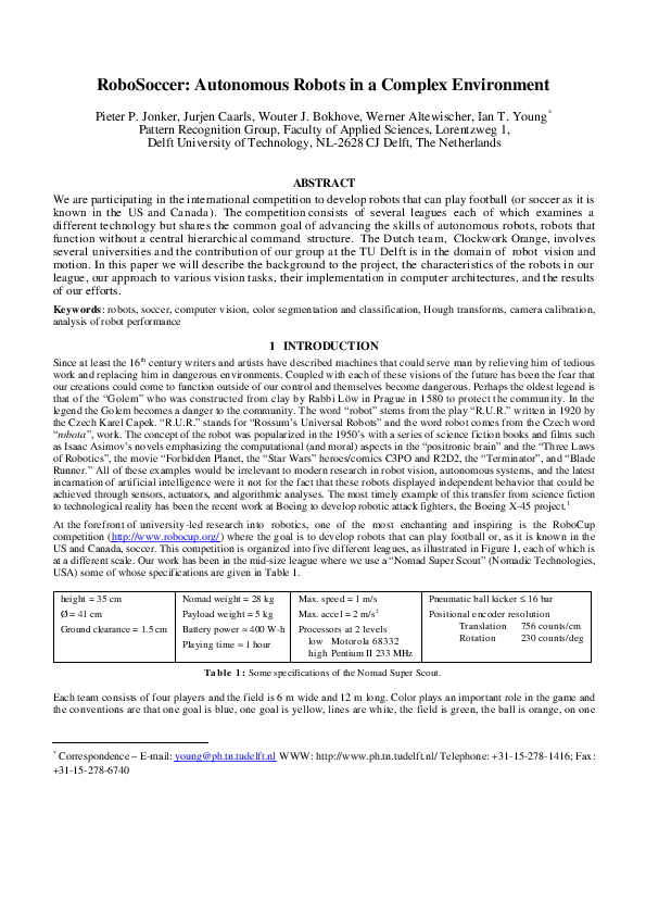This competition is organized into five different leagues, as illustrated in Figure 1, each of which is at a different scale. Our work has been in the mid-size league where we use a “Nomad Super Scout” (Nomadic Technologies, USA) some of whose specifications are given in Table 1. height = 35 cm Nomad weight = 28 kg Max. speed = 1 m/s Ø = 41 cm Payload weight = 5 kg Max. accel = 2 m/s 2 Ground clearance = 1.5 cm Battery power ≈ 400 W-h Processors at 2 levels low Motorola 68332 high Pentium II 233 MHz Playing time ≈ 1 hour Pneumatic ball kicker ≤ 16 bar Positional encoder resolution Translation 756 counts/cm Rotation 230 counts/deg T a b l e 1 : Some specifications of the Nomad Super Scout. Each team consists of four players and the field is 6 m wide and 12 m long. Color plays an important role in the game and the conventions are that one goal is blue, one goal is yellow, lines are white, the field is green, the ball is orange, on one * Correspondence – E-mail: young@ph.tn.tudelft.nl WWW: http://www.ph.tn.tudelft.nl/ Telephone: +31-15-278-1416; Fax: +31-15-278-6740 team the players wear magenta shirts, and on the other team the players wear cyan shirts. This is illustrated in Figure 2 both schematically and with a color photo of part of the playing field. (a) (b) (c) (d) (e) F i g u r e 1 : (a) Simulation league based solely upon a computer simulation of two opposing teams and involving no physical robots; (b ) small-size league involving “Lego-like” robots; (c ) four-legged league involving “puppy-like” robots currently manufactured by Sony; (d) “mid-sized” league whose height and width can be around 40 cm; (e ) humanoid league intended to mimic human size and bipedal motion. (a) (b) (c) Figure 2: (a) Standard playing field with four players on each team; (b ) the Nomad Super Scout robot as delivered from the factory; (c ) two players from one team in magenta and two players from the opposition in cyan. The green field, white lines, and orange ball are clearly visible. 2 INTERACTION WITH THE ENVIRONMENT It is important to understand that each robot, while it listens to the reports from the three other team players and the “coach” using wireless Ethernet, operates as an autonomous unit. The two actions that it can execute, movement or kicking, are not the result of orders from a “military-like” hierarchical command structure, but rather based on its evaluation of its “world picture” derived from the information it receives from others as well as from its own measurement sensors. Each robot has two types of measurement sensors, odometry sensors for position and a 1-chip color CCD camera for robot vision. Each robot is capable of translational and rotational motion and of kicking the ball with a specially-designed pneumatic mechanism. All motion is accomplished through a two-wheel differential drive, visible in Figure 2b, whose geometric center is at the center of the physical robot. The positional sensors measure the distance that the robot has traveled in a specific translation as well as the angle through which it has turned during a rotation. The specifications of these two sensors are described in Table 1. The color camera that has been used is a Chugai NTSC camera model YC-02B and is shown in Figure 3b. The camera has automatic white balance as well as automatic gain control. Because of the constrained and highly specific way in which colors are used in this environment, we have disabled the automatic white balance and, instead, provided an absolute white reference shown in Figure 3b. The lens used with the camera has a 94° field of view and good depth-of-field. The frame grabber is a WinTV PC model used to provide 320 x 240 pixel images where each pixel is composed of {r, g, b} values each of which is eight bits deep. (a) G R G R B G B G G R G R B G B G (b) (c) (d) Figure 3: (a) Nomad Super Scout including computation, vision, communication, and ball-handling modules (b ) Detail of the vision module showing the camera, the 94° wide-angle lens, the anti-glare polarizing filter and the absolute white reference; (c ) the 1-chip CCD camera leads to coarse-grain sampling of red and blue and medium-grain sampling of green; (d) the effect of the color sampling is shown in the color distortion in the sampling of the white lines. CCD cameras that use only one chip are known to have problems in providing sufficient color resolution at every spatial coordinate. This problem is illustrated in Figure 3c,d where the lack of {r, g, b} information at every pixel lead to errors at the edges of the white line in the image of the playing field. It is to be expected that developments in camera technology (e.g. Foveon cameras2) will eliminate this problem in the future but for now we must deal with it. A polarizing filter is also visible in Figure 3b and this is used to reduce the effects of glare and specular reflections from various objects including the ball whose surface, as shown in Figure 4, is quite glossy. dribble F i g u r e 4 : The glossy surface of the ball is evident. The kicking mechanism as well as the mechanism for transporting the ball across the field (“dribbling”) can also be seen. kick 3 CALIBRATION Using a standard white reference card instead of the built-in automatic color balance is one example of what we consider to be calibration. Within the domain of robot vision several other calibrations steps are required to compensate for geometric distortion due to camera tilt and the use of a wide-angle lens (94°). Further, even if both of these distortions were absent there would still be the change in the measured size of objects as a function of their axial distance to the camera lens. Each of these is problems is addressed in a different way. The “tilt” comes from the fact that the camera, sitting at a height of some 40 cm above the floor, does not have a line-ofsight parallel to the floor but rather looks down at an angle of about 45°. This can be seen in Figure 3a,b. The tilt produces a parallax distortion which can be corrected by standard techniques from projective geometry. Three parameters must be estimated in a calibration step before a game begins: the focal length ƒ of the lens, the angle ϕ that the camera lens makes with the horizon, and a vertical distance measure Y CCD in the plane of the CCD chip. With these numbers the non-linear mapping of the original coordinate geometry to the corrected geometry can be computed and loaded into look-up tables to permit correction for the tilt effect before a game begins. During an actual game the use of look-up-tables provides for highspeed tilt correction. The use of a wide-angle lens means that a form of radial distortion occurs in the image. While for a normal lens this effect would be negligible, in our case the distortion is not acceptable. This problem has been studied in-depth by Tsai3 and we have implemented his solution in the form of look-up tables. Again, this correction requires a pre-game calibration step. The use of the look-up tables is illustrated in Figure 5a,b and the results are shown in Figure 5c,d. (a) (b) (c) (d) F i g u r e 5 : Correcting for radial distortion. Pixels for which no image information is available after application of the coordinate transformation are shown in red. (a) correction terms for the horizontal component in the look-up table; (b ) correction terms for the vertical component in the look-up table; (c ) distorted original scene; (d) distortion removed after application of the Tsai algorithm. Another “distortion” is caused by the apparent decrease in size of the ball as its distance to the camera gets larger. We calibrate for this by first using our prior knowledge about the actual size of the ball and then calculating what its size would be for every possible location of its center y coordinate in the image. This yields a matrix of expected radius r versus y which can (again) be used in a calibration look-up table to analyze the image. This effect is illustrated in Figure 6 where two soccer balls are simulated on a grass field. In Figure 6a we see the two orange spheres as approximately equal in size. But when the camera viewpoint is changed to a position similar to that of our robot camera, as shown in Figure 3a,b, this results in the situation depicted in Figure 6b. The two spheres are no longer of the same size and the tilt of the camera places the sphere that is closer to the camera as lower in the image. This correlation between size, expressed in a radius r, and vertical position in the image, as expressed as y, is the basis of a mechanism to estimate the position of the soccer ball that will be described below. (a) (b) Figure 6: Simulated environment for analyzing the relationship between perceived size and position in a projected image (a) two soccer balls in a 3-D environment; (b ) the two soccer balls as seen from the robot camera position. In summarizing, all three of the distortions described above are handled by a combination of calibration steps that are taken before a game and then implemented in correction look-up tables during a game. 4 IMAGE SEGMENTATION Our strategy for analyzing the images in real time is to first classify every pixel on the basis of its color into one of several classes: playing field (green), ball (orange), goal (yellow), goal (blue), lines (white), team players (magenta or cyan), opposition players (cyan or magenta), and robot bodies (black). While the color space provided by the camera is {r, g, b} a more appropriate space might be {h, s, i}. Unfortunately, the mathematical transformation from {r, g, b} to {h, s, i} in software would take too much time and the hardware chip to do this would involve an extra circuit board which would cost us energy and, as indicated in Table 1, our energy budget is strictly limited. We have chosen, therefore, to use a modified form of the {y, u, v} color space which we refer to as {y’, u’, v’}. The transformation is given by: y'  1    u' =  1 v'  0    1 1  r     −1 0  • g  −1 1  b  (1) and only additions and subtractions are required to produce this representation. The actual color information is contained in the coordinates u’ and v’. The division of this two-dimensional color space into classification regions is based on a “piechart” approach, where different angular regions are considered as describing the colors associated with certain objects. The steps in this pixel classification scheme are shown in Figure 7. v’ u’ (a) (b) (c) Figure 7: Pixel classification using {u’, v’} (a) an original color scene; (b ) the position of each pixel in {u’, v’} space; (c ) the result of classification and labeling with a pseudo-color. The next step is to go from classification at the level of pixels to finding the objects (lines, goals, ball, etc.). To accomplish this, a fast, intermediate step is used to find regions-of-interest (ROIs) where we can expect with a reasonable certainty that the objects will be found within the pixel-classified image. The basis of this step is the use of projection histograms, a tool that was developed and used more than 30 years ago. The basic concept is illustrated in Figure 8 for two of the class labels, orange (ball) and black (robot). Looking across each row, i, we sum the number of pixels that have been labeled with a specific color. On the third row in Figure 8, for example, we see that there is a total of two orange pixels and three black pixels. Continuing this for all rows and all columns we thus compute two “orange” histograms (one for the columns and one for the rows) and two “black” histograms. This procedure is, of course, not limited to just these two colors but is instead applied to all the colors in our labeled image except green; we do not need to know where the playing field is. ↓ Projection i i→ j↓ 0 3 3 0 0 4 4 0 0 0 2 0 3 0 4 2 1 2 0 2 0 4 0 2 0 2 0 0 0 0 0 2 3 2 0 0 2 1 0 0 ← Projection j Figure 8: Projection histograms for two of the colors and for the rows and columns associated with each color. We now filter these histograms to reduce the effect of noise and then determine the ROIs. The filtering algorithm is a straightforward two-step operation and illustrated in Figure 9. 0 2 0 1 0 1 3 3 1 1 1 1 3 2 1 1 1 1 0 0 0 0 0 0 0 0 → 0 0 → 0 0 4 2 Value in cell > 1 1 1 2 out of 3 consecutive entries > 1 1 0 4 1 1 0 1 0 0 0 0 0 0 0 0 0 0 0 0 0 (a) step 1 (b) step 2 (c) (d) Figure 9: Filtering projection histograms (a) original row histograms taken from Figure 8; (b ) thresholded histograms; (c ) 2-out-of-3 filtered result; (d) ROIs identified for objects in the image. The colors of the rectangular boundaries have no special significance and are only intended to make the ROIs visible. The first step in filtering the histograms is thresholding. Histogram values greater than one (> 1) in the projection histogram (Figure 9a) are set to one; otherwise they are set to zero. The second step is to look at three consecutive values of the thresholded result as shown in Figure 9b. If less than two (< 2) of the entries are one then the center value in the window of three is set to zero; otherwise it is set to one. The result in Figure 9c shows that two objects have been found in the black-labeled image and one object has been found in the orange-labeled image. By “found” we mean that a rectangular ROI has been identified around labeled objects, their labels are still known, and noise-like objects have been rejected. An example of applying such a projection histogram procedure is shown in Figure 9d where the nine ROI bounding boxes are indicated in arbitrary colors. The final step is classification of the objects within the ROIs. 5 OBJECT CLASSIFICATION The label derived from the color segmentation and now attached to a ROI gives a reasonable estimate of what object can be found inside the ROI. Playing soccer, however, requires more information. We must be able to move to the ball. We must know where the goal is, where the boundary lines of the playing field are, and the status of the other robots that we have seen. Are they on our team or part of the opposition? The principle tool that we use, in addition to color, to identify an object inside a ROI and determine its parameters is the Hough transform. This well-known technique4 allows us to determine which objects are straight lines and which are circles. The former is essential if we are to know where we are in the absolute coordinate system of the playing field. The odometry measurements are not sufficient for this as it is too easy for the robot to lose its position with the relative information provided by the position encoders. (This can happen, for example, when a robot “spins its wheels” after collision with another object.) Our implementation of the Hough transform for straight lines is standard and will not be elaborated upon here. Our implementation of the Hough transform for circles takes into account the fact the we do not know the radius of the circular object that we are seeking but, if we can find the center coordinates of the ball (Xc , Y c ), then knowledge of Y c together with our knowledge of the true radius of the soccer ball will tell us where the ball is on the playing field. We proceed as illustrated in Figure 10. We generate an image of the contour pixels on the orange object inside the ROI. We start with a guess of the ball’s radius based upon its possible y position in the playing field as illustrated in Figure 6b, that is, we choose a (weighted) average starting estimate for Ro. We now apply the Hough transform to the representation of a circle using the two-parameter model: ( x − Xc )2 + ( x − Yc) 2 = R2o (2) The transform space is now characterized by (Xc , Y c ) and for each pixel on the contour we obtain a circle in the new space. Using peak detection in the parameter space leads to the most likely value for the center coordinates of the ball. We now proceed to that position in the calibration image that provides a revised estimate of the proper value of R at that position y = Y c and then using the revised estimate for R = R1, we repeat the Hough procedure. This converges quickly to a satisfactory estimate of the position of the ball on the playing field. This iterative procedure is summarized in Figure 10. update radius estimate center of ball iteration default radius Circular Hough transform (a) (b) F i g u r e 1 0 : Circular Hough transform for ball finding (a) an iterative procedure starts with an estimate for the ball’s radius. This is updated on the basis of the ball’s “vertical” position in the image; (b ) the ball’s position indicated by the black circle and the two field lines indicated by the red lines as found using Hough transforms. 6 COMPUTER STRATEGIES It is obvious that all of the computations must be done in the most time-efficient and energy efficient manner possible. To accomplish this we have looked at the use of two different types of processors for the image processing and analysis. These two processors are an Intel Pentium processor running at 233 MHz and a 40 MHz IMAP Processor board (NEC Corporation, Kawasaki, Japan). The former is a general purpose processor running under Linux Red Hat v5.2. The latter is a board containing 8 special chips each of which in turn contains 32 processor elements (PEs) for a total of 256 PEs on a single board. The Pentium architecture is well-known; a detailed description of the IMAP board can be found in vd Molen et al.5 and a picture of the layout is shown in Figure 11. Figure 1 1 : IMAP-Vision board with 8 x 32 processor elements. The IMAP is significantly faster than the Pentium as the figures in Table 2 show. But the IMAP also uses a considerable amount of current and it is not possible to replace the Pentium with the IMAP. The Pentium is needed for the motion, communication, and kicking systems. The IMAP can only serve as an additional processor dedicated to image processing tasks. We therefore have to consider the situations where it is appropriate to make use of this technology. The Pentium uses a certain average amount of power. The three Nomad robots that move over the entire playing field also consume a significant amount of energy in the course of a game through their mechanical actions. The goalie robot, however, has only a limited amount of mechanical motion but needs quick visual “reflexes” to defend the goal. As a result we have equipped the goalie with the IMAP-Vision system. The other three robots must rely on the Pentium for their image processing. A comparison of the effectiveness of these two architectures is given in Table 2. Pentium with 64 MB RAM 233 MHz clock frequency IMAP-Vision with 256 processors 40 MHz clock frequency Color classify objects 10 ms 7.7 ms Find ROIs 10 ms 2.6 ms Circular Hough transform 50 ms 3.9 ms Linear Hough transforms 50 ms 4.2 ms Find playing field corners 2 ms 2.1 ms Process T a b l e 2 : Comparison of the two processors on the same tasks. These are somewhat specialized tasks. When a 300 MHz Pentium II with MMX architecture was compared against the same IMAP-Vision card on a suite of standard image processing algorithms (e.g. add, AND, 3x3 convolution, Sobel, dilation, etc.), the IMAP-Vision was 10 times faster. Both architectures have been updated and the latest version of the IMAP card remains at least 5 times faster than the latest Pentium architecture.6 7 SUMMARY AND CONCLUSIONS The actual effectiveness of our approach must be judged not by the speed of individual algorithms but the performance at tasks. The detection of all major objects is good with the weakest aspect being the detection of the black robot bodies. The color black also means “no signal” which in turn means a poor signal-to-noise ratio in the relevant pixels. The color classification is fine with the only problem being in the recognition of the team colors, magenta and cyan. Angular measurements are accurate to within 1°. Distance measurements are accurate to within 5% meaning 5 cm at a distance of 3 meters and 2 cm at a distance of 40 cm. This latter figure is important in ball-handling. The image processing algorithms take an average of 26% of the Pentium processing capacity when images are analyzed at 15 fps. (This is the rate that has been chosen in using images of 320 x 240 pixels.) The remaining capacity is available and needed for the other aforementioned tasks. Our team “Clockwork Orange” has not as yet won any championships but there has been a marked improvement in our performance. In the June 2001 German open we lost 2 games and tied 2 games. We scored 0 goals and the opposition scored 7. Two months later at the World Cup competition we won 4 games, tied 1, and lost 3. Our goal balance changed even more dramatically; we scored 16 goals and the opposition 17. There are many components of a soccer team that are outside the scope of image processing such as motion strategies and team strategies. All of these must be addressed to have a successful team. At this moment we are reasonably satisfied with the image processing components although we hope to improve the speed and accuracy of all of our visual detection tasks. ACKNOWLEDGMENTS This work was partially supported by the Delft University of Technology, the Philips Center for Fabrication Technology, Dr. Sholin Kyo and the NEC Incubation Center in Kawasaki, Japan, and the Dutch Ministry of Economic Affairs through the Senter program “IOP Beeldbewerking”. We gratefully acknowledge their support. REFERENCES 1 Russ Mitchell, “The Pilot, Gone. The Market, Huge,” in New York Times in Business section (New York, 31 March 2002), pp. 1-2. 2 John Markhoff, “Digital Sensor Is Said to Match Quality of Film,” in New York Times in Business Financial section (New York, 11 February 2002), pp. 1. 3 Roger E. Tsai, “A Versatile Camera Calibration Technique for High-Accuracy 3D Machine Vision Metrology Using Offthe-Shelf TV Cameras and Lenses,” IEEE Journal of Robotics and Automation, RA-3:4, pp. 1987. 4 P.V.C. Hough, Method and means for recognizing complex patterns, Patent # 3069654, USA, (1962). 5 M. vd Molen, S. Kyo, and W. Bokhove, Documentation for the IMAP-VISION image processing card and the 1DC language, NEC Incubation Center, Kawasaki, Japan, 1999. 6 S. Kyo, T. Koga, and S. Okazaki, “IMAP-CE: A 51.2 GOPS video rate image processor with 128 VLIE processing elements,” presented at ICIP-2001, Thessaloniki, Greece, Editor(s): I. Pitas, M. Strintzis, G. Vernazza et al. ed., pp. 294297, 2001.