zyxwvu zyxwvut zyxwv zyxwvutsr zyxwvut Langmuir 1993,9, 2523-2529 2623 The Brunauer-Emmett-Teller Equation and the Effects of Lateral Interactions. A Simulation Study Alon Seri-Levy and David Avnir’ Department of Organic Chemistry and the F. Haber Research Center for Molecular Dynamics, The Hebrew University of Jerusalem, Jerusalem 91904, Israel Received June 18,1992. In Final Form: November 1 0 , 1 9 9 9 Adsorptionldesorption on a smooth surface is studied at the molecular level by new, simple two-dimensionalMonte Carlo simulation procedures using site-specificadsorptiorddesorption probabilities. The classical BET conditions are simulated and the resulting adsorption isotherms show a very good fit with the calculated theoretical parameters of the equation. The BET islands are visualized and analyzed. Following this test simulation, lateral interactions are added, resulting in type I1 and type 111isotherms. The ensuing deviations from BET behavior are identified and analyzed. It is shown that accurate surface area values can only be obtained from an unequivocal B-point. The effects of changes in adsorption1 desorption probabilities on the isotherm shapes are identified and discussed. The changes in the heat of adsorption with coverage are analyzed. It is found that this type of plot is a very sensitive analytical tool for locating the monolayer value. 1. Introduction zyxwvu roughness factor is 1.0 in order to be able to make a direct comparison with the BET monolayer value.4 Molecular level computer simulations of adsorption processes are devoid of this problem. Since here the true surface area is a known input, it is possible to test the accuracy of the BET equation under the more realistic conditions of lateral interactions and an energetically heterogeneous surface (the effects of the latter to be addressed in a subsequent report). The usefulness of computer simulations to the understanding of surface science is by now well documented.”12 What had been thought to be a disadvantage, namely the inability of simulations to provide true-to-life mimicry of all parameters involved, turned out to be an advantage: one can identify, isolate, and study single important parameters, free of the fogginess imposed by real conditions. The approach adopted here is, we believe, novel and concentrates on adsorption/desorption probabilities at the single molecule level. Its main advantages are as follows: (a) It allows convenient simulations of adsorptionldesorption processes on irregular morphologies of any shape and form13 which are either very difficult or impossible to perform by classical simulation methods (these morphologies are the topic of a subsequent reportI4). (b) It allows the visualization of the adsorption process on a molecular level: in a sense, our approach provides molecular level microscopy for such processes. (c) We show that the very basic and elementary rules are capable of retrieving quite A paper written by Brunauer shortly before his death provides a rare glimpse into the bitterness with which this forefather of surface science looked back upon his lifetime career.’ He opened his paper with “I am not sure that there is a paper in the last half century that produced as much adverse criticism as the BET2paper”, and ends his account with “[Langmuir’sl equation was one of the reasons for getting his Nobel Prize”, whereas “The BET paper was recommended for the Nobel Prize but did not receive it.” Adds Adam~on:~ “However, it is still, after almost 50 years, among the most frequently quoted papers in the field. As for practical applications, suffice it to say that one place alone, the Institute of Catalysis at the USSR Academy of Sciences, makes some ten thousand BET surface area measurements per year.” This fascinating dichotomyof the BET equation reveals an important face of the modern scientific method: the ability to achieve tremendous progress in a field, using a theory that far from reflects reality. In a sense, the BET equation is a monument to the achievements of imperfection. The main criticism of the BET model is that it uses two basic assumptions that are intrinsically inaccurate. The first is that all adsorbing surface sites are assumed to be energetically homogeneous, and the second is that only vertical interactions between adsorbed molecules and the adsorbent surface take place, thus neglecting lateral (horizontal) interactions between adjacent adsorbed molecules. In the light of these basic (and problematic) (4) Lowell, S.; Shields, J. E. Powder Surface Area and Porosity, 2nd assumptions, the key question asked about the BET ed.; Chapman and Hall: New York, 1987. equation is whether the surface area measurement it (5) Nakagawa, T. Kolloid 2.2.Polym. 1967,221,40. provides is the “true”,correct value. Althoughthe general (6) Steele, W. A.; Bojan, M. J. Pure Appl. Chem. 1989,62,1927. (7) Morioka, Y.; Kobayaehi, J.4. Nippon Kagaku Kaishi 1982, 549. concensus seems to be that the answer is negative, it has (8) de Keizer, A.; Michalski, T.;Findenegg, G.H. Pure Appl. Chem. been impossible to evaluate by how much the BET area 1991.63.1495. - ..-, - -,- ._ -. is off, since there has been no method that could (9) Citri, 0.;Kagan, M. L.; Kosloff, R.; Avnir, D. Langmuir 1990, 6, 569 (Erratum: 1991, 7,610). independently provide that elusive “true” value. Even in (10) Seri-Levy, A.; Avnir, D. Surf. Sci. 1991,248, 268. calculations using “perfect” crystals with a known geo(11) Patrykiejew, A.; Binder, K. Surf. Sci. 1992,273, 413. metric area, the assumption had to be made that the zyxwvutsrqponmlkjihgfedcbaZYXWVUTSRQPONMLKJIHGFEDCBA (12)Nicholson D.; Parsonage, N. G. Computer Simulation and zyxwv ~~~ Abstractpublished in Advance ACS Abstracts, August 15,1993. (1)Brunauer, S. Langmuir 1987,3,3. (2) Brunauer, S.; Emmett, P. H.; Teller, E. J. Am. Chem. SOC.1938, 60,309. (3) Adamson, A. W. note 7 in ref 1. 0 Statistica~hfechanicsof Adsorption; Academic Prese: London, 1982;pp 328-342. (13) (a) Seri-Levy,A.; Avnir, D. Proceedings of the 4th International ConferenceFundamentale of Adsorption, Suzuki M., Ed.,in press. (b) Seri-Levy, A. PbD. Thesis, The Hebrew University of J e d e m , Jerusalem, December 1992. (14) Seri-Levy, A.; Avnir, D. Preprint, 1992. O743-7463/93/24O9-2523$04.oO/o 0 1993 American Chemical Society zyxwvutsrqponm zyxwvutsrqp zyxwvutsrq zyxw zyx zyxwv Seri-Levy and Avnir zyxwvutsrq 2524 Langmuir, Vol. 9, No. 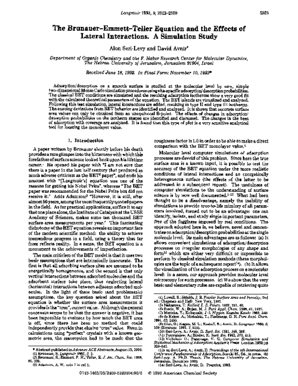10, 1993 ooo 0 m o 0 ,”, 00 m m 0 O o 00 9 ,m O 00 0 0 o oo9 o 00 E 8 0 0 ’ 00 m o o 0 00 O 0 00 oo o o ooo oooo 000 0 0 0 oo m 08 00 0 0 o 0 0 0 0 0 , ” ” 0 Figure 1. Tower-like structure of the BET islands: surface, 0; adsorptive or neighboring molecules, 0;adsorbed molecules, 0 . Net adsorption probabilities: A l / D l = 19, Az/Dz = 3. PIP, from bottom to top: 0.13, 0.27,0.41, 0.55. accurately realistic shapes of adsorption isotherms and realistic changes in their shapes, as adsorption parameters are varied. The main aim of this study was to construct a Monte Carlo molecular level simulative procedure of adsorption/ desorption processes, with lateral interactions. This was achieved by first simulating the classical BET equation, retrieving all its parameters, and subsequently adding lateral interactions. Mimicking the BET model of the adsorption/desorption process before adding the lateral interactions ensures that the revised algorithm is free of artifacts. In addition to the estimation of surface area using the BET equation, the B-point method was also employed for the resulting isotherms, and guidelines for increasing the accuracy of the BET monolayer prediction ability under conditions of lateral interactions are suggested. The simulation of the original BET model also allows one to observe, perhaps for the first time, the unnatural arrangement in “islands” of the adsorbed molecules on the surface. We finally expkorethe potential use of average adsorption probabilities for the analysis of surface heterogeneity. 2. Details of the Computer Simulations 2.1. General Properties. The conducted simulations were two-dimensional and of Monte Carlo type. In all simulations, the surface was a line 100 pixels long (Figure 1,hollow squares). A reservoir (square lattice), 100 pixels wide, was placed above the surface and contained an initially homogeneously-distributed amount of adsorptive molecules (ideal gas), each molecule occupying an area of 1 pixel. A reservoir pixel can be either empty or occupied with no more than one adsorptive in it. At any moment, three types of molecule populations can be found (Figure 1): adsorbed molecules (black circles); neighboring molecules, unadsorbed molecules which are adjacent either to a surface site or to an adsorbed molecule, and hence available for adsorption in the next time step (hollow circ1es);gasphase molecules, unadsorbed molecules which are not available for adsorption in the next time step (also hollow circles). Accordingto the BET model, only vertical interactions are possible and hence an unadsorbed molecule will be considered as a neighboring molecule only if it is located on the top (position [ x , yl) of either a surface site or an already adsorbed molecule (located in position [ x , y - 11). In the case of lateral interactions, the population of neighboring molecules is extended. Here the “top” limitation does not exist, and an adsorbed molecule or surface site in any one of the positions [ x , y + 11, [ x + 1, y], or [ x - 1,yl will also bring the unadsorbed molecule at position [ x , y ] into the definition of “neighboring molecule”. 2.2 Simulations of the BET Conditions. The simulations of the BET test case were carried out as follows. At each time step, all molecules are treated consecutively in random order. A selected molecule may belong to one of the three populations mentioned above and, accordingly, undergoes one of the following: If the chosen molecule neighbors a surface site or an adsorbed molecule, adsorption is attempted with probabilityA1or A2, respectively. If successful,this neighboring molecule becomes adsorbed. If unsuccessful, it remains in place. If the chosen molecule is adsorbed on the surface or above another adsorbed molecule, with no adsorbed molecule on top of it, desorption is attempted with probability D1 or Dz,respectively. If successful,it becomes a neighboring molecule. If unsuccessful, it remains in place. After all the molecules have been treated, all gas-phase molecules and neighboring molecules (all hollow circles) are mixed and redistributed randomly and homogeneously, and the next time step begins. This procedure is repeated until equilibrium is reached, i.e. until the amount of adsorbed molecules remains constant for at least lo00time steps. For a full adsorption isotherm, the whole procedure is repeated for various initial gas-phase concentrations. The value of PO, the “saturation” concentration or pressure, is calculated from DdA2 as explained below (eq 7). 2.3 Simulations with Added Lateral Interactions. The addition of lateral interactions diminishes the distinction between adsorption to the first layer and to higher layers. For each set of simulations, two interaction heats are defined. The first, Q1, is defined as the heat of adsorption to the surface, and the second, Qz,is defined as the heat of interaction between two adjacent adsorbed molecules (heat of liquefaction). In thermodynamic terms, the net probability of adsorption to the first layer, A1/D1, is exp(Q1lRT) and to higher layers, AzlDz, is exp(Q$RT). Hence, by adding lateral interactions of van der Waals type, the net adsorption probability, either to the first layer or to any higher layer, is zyxw zyx A - = exp((ZIQl + Z,Q,)/RT) (1) D where 21 is the number of nearest neighboring surface sites (21 = 1 in the case of smooth line) and 22 is the number of nearest neighboring adsorbed molecules. The temperature, T, is also an input parameter of the simulation. For purposes of economizing in computer time, A was defined as A = 1,and D was determined by the input values of Q and T, according to eq 1. zyx zyxwvutsrq zyxwv Effects of Lateral Interactions zyxwvutsrqponmlkjihgfedcbaZYXWVUTSRQPONMLKJIHGFEDCBA Langmuir, Vol. 9, No. 10,1993 2625 Figure 2. An artist’s (A. W. Adamson) visualization of Figure 1. Reprintedwithpermissionfrom ref 15. Copyright 1990Wiley. 1.0 ! I 0 5 0 I 15 10 20 Island Size (pixels) Figure 4. Distribution of BET islands obeys eq 2. The results for 90 lines of 100 pixels each were summed up. AdD1 = 19, AdDz= 3,PIP, = 0.41 (taken at equal time intervals of 100time steps at equilibrium). In addition to the maintenance of constant pressure for 1000 time steps, equilibrium conditions were doubly ensured by examining the size distribution of the BET islands. The latter should obey a simple law which is derived as follows: Taking the fraction of occupied sites to be 1- Bo, we ask what is the probability of obtaining, within the randomly distributed occupied sites, an island of width k. Since 1- 80 is the probability of finding an occupied site, then the probability of finding a sequence of k neighboring sites is (1- Bo)c. An island is bound by two empty sites, and hence the probability of finding an island of size k is (1- Bo)kBo2. If the totalnumber of surface sites is Mt, then the total number of islands of size k is zyxwvu zyxwvu zyxwvut zyxwvut kfk= ~ , -( eo)ke,2 i Figure 3. Equilibrium dynamics of BET islands during 30 consecutive time steps (left column from top to bottom then right column from bottom to top). Al/D*=19,AdDz = 3,PIP0 = 0.41. 3. The BET Equation 3.1. The BET Islands. The BET simulationsnot only serve as a test case but also provide an opportunity to obtain a visual display of the BET islands. To the best of our knowledge, this very basic aspect of the BET equation has not been reported. One does find intuitive descriptions of these adsorbed patches, such as that provided by Adamson15 (Figure 2), but not computed islands. Figure 1shows the picture for the set A1/D1= 19, AdDz = 3 at four PIP0 (=m/mo,where m is concentration) values and the increase in the size and height of the islands as the pressure is increased. Interestingly, on the molecular islands, Brunauer wrote: “Teller ...felt-very justly-that the model of columns of different heights of molecules is not right”.’ The dynamic nature of the BET islands at equilibrium is demonstrated in Figure 3 for 30 consecutive time steps, for the same PlPo value. The reader is invited to follow one of the islands through the 30 time steps in order to get a first-hand impression of the structural changes that occur within it. From Figure 1one can see that Teller’s doubts were justified, especially at high concentrations. Adding lateral interactions (as will be demonstrated below) flattens the BET islands into more realistic shapes. (15) Adamson, A. W .Physical Chemistry of Surfaces, 6th ed.; Wiley: New York, 1990;p 611. (2) A plot of In Mk vs k should give a straight line. As can be seen in Figure 4, this equation is nicely obeyed, with Bo = 0.206 from the intercept and 00 = 0.204 from the slope, compared to the value of 0.189 as obtained by the direct counting of sites. The cumulative data of 90 equilibrium steps is shown. 3.2. The BET Isotherm. The comparison between the simulation results and the BET theory is made as follows: a,the ratio between 81, the coverage by one layer of adsorbed molecules, and the uncovered surface Bo, is given by B1 k’A,P a=-=-=00 4 1 kAlm VlDl (3) where k’ is a constant counting the number of collisions per unit time per unit area normalized to the pressure, and v1 is the vibration frequency of the adsorbates. Since we perform our simulations in terms of concentration, m, rather than P, k replaces k’. A neighboring molecule collides (attempts an adsorption) only once in each time step. The average rate of collisions per surface site is, however, less than 1, by a factor determined by the concentration of the neighboring molecules. Since this value is normalized to the total concentration which, in turn, is equal to the concentration of the neighboring molecules, k = 1. Similarly, VI = 1 because at each time step the adsorbate makes one attempt to desorb. Equation 3 then simplifies to zy zyxwvutsrqpon zyxwvutsr Seri-Levy and Avnir 2526 Langmuir, Vol. 9, No. 10,1993 theoretical and simulation results. The dashed line is the BET function in the form where N is the number of adsorbed molecules and Nmis the monolayer value. N, is known (=loo) and C is calculated from eq 6 and given in Table I. It is seen that as C increases, the simulation is able to reproduce the expected change in the isotherm shape. Figure 1shows the actual molecular distribution at several P/Povalues on one of these isotherms. Figure 5b shows the fit of the three isotherms to the BET equation zyxwvutsrqpo --+-(-) c-1 (10) N[(P,,/P) - 13 NmC NmC Po Notice that since the equation (and consequently its simulation) is free of lateral interactions and condensation, the fit is not limited to the 0.05-0.3p/p0range but can be carried out to higher PIP0 values. Table I shows the comparison between the calculated parameters (eqs 6 and 8) and the simulation results (eq lo), and the agreement is good. Having analyzed these simulations of the classical BET isotherm equation, and having demonstrated that our simulation conditions accurately retrieve this equation and mimic equilibrium states, we proceed to more realistic adsorption conditions. 1 1 P P I Po zyxwvutsrqponmlkjihgfedcbaZYXWVUTSRQPONMLKJIHGFEDCBA - " zyxwvutsrqponm zyxwvutsrqpo zyxwvutsrqpon b 011 012 013 014 015 016 017 018 PIP, Figure 5. (a) BET adsorption isotherms. The parameters are collectedin Table I. Isotherms a, b, and c refer to bottom, middle, 0 , and 0 are the simulation and upper lines, respectively. ., results. The dashed lines are the fit of these results to the BET equation (eq 9). Figure 1 shows four equilibrium points on isotherm a. (b) BET analysis (eq 10)of the isotherms in a. The resulting parameters are shown in Table I. (4) Similarly 4. Adsorption with Lateral Interactions 4.1. The Adsorption Isotherms. The BET equation, as will be recalled, does not take lateral interactions into account, although these cannot be neglected in most, if not all, adsorption processes. Isotherm equations including lateral interactions have been suggestedl6J7but never gained wide use. Instead, the BET equation is universally used, at least in the sense that all manufacturers of adsorption instruments install the equation as the standard automated way to evaluate surface area. Perhaps the main reason for this situation is the fact that quite often, analysis of experimental data according to eq 10, over the traditionally recommended PIP0 range of 0.05-0.3,does provide a good straight line. With the popular single-point BET determinations, there is clearly no fitting whatsoever. It is the aim of this section to estimate the error involved in BET surface area determinations, to find under what conditions eq 10 appears to work in the presence of lateral interactions, and to see how one can minimize BET errors in such cases. Figure 6a shows a set of five adsorption/desorption isotherms for which QdRT = 0.5195 and Q1/RT decreases gradually from 12.987 to 0.649 (curves a-g, respectively). The following observations and interpretations are made: No hysteresis of the adsorption/desorption loop is observed. This is an important test since we show in a subsequent report that introduction of geometric irregularity is sufficient for the full development of such hystereses. This test also corroborates the fact that in our simulations a good equilibrium state is obtained at each point. For the four highest QlIRT values, i.e. strongest adsorption, the classical type I1isotherm is obtained (Figure 6a, curves a-d). We recall that this shape of isotherm is typical for adsorptions on nonporous or macroporous zyxwvutsr where B1,, B,, are the fractions of surface covered by columns of n - 1and n adsorbed molecules, respectively. The BET constant, C, can be calculated from eqs 4 and 5 This equation allows comparison between the C obtained from the simulation and the calculated one. Finally, since under BET conditions4 (7) where mo is the saturation concentration, mo can be calculated from eqs 5 and 7 mo = D2/A2 (8) The BET simulations were carried out for three pairs of A1/D1, Ad02 values. The three resulting isotherms are shown in Figure 5a, with an excellent agreement between (16)Hill, T. L. J. Chem. Phys. 1947,16, 767. (17)Gregg, S.J.;Sing,K. S. W. Adsorption, Surface Area andPorosity; Academic Press: London, 1982. Effects of Lateral Interactions zyx zy zyx zyxwv Langmuir, Vol. 9, No. 10,1993 2627 zyxwvutsrqp Table I. Simulation of the BET Conditions experimental results zyxwvutsrqponmlkjihgfedcbaZYXWV BET prediction input values BET PIP0 zyxwvutsrqpo Po isotherm (Figures 5a,5b) a, 0 N,cP from AdD1 AdDz (~oP Cb simulation 101 19 3 113 6.3 100 213 12.7 19 1.5 b, 0 100 213 132.7 C, 8 199 1.5 F’rom eq 8. * From eq 6. Using eq 10. Input value: N , = 100 pixels. 250 i: c f 200 a a 150 ”c 100 4 i2 50 0 0 0.1 0.2 0.3 0.4 0.5 0.6 0.7 PIPo - 0.002 FE 5 0.001 0 PIPo Figure 6. (a) Adsorption isotherms with QdRT = 0.5195 and lateral interactions: 0,adsorption; 0 , desorption. From top to bottom (a-g): QdRT = 12.987,7.792,5.299,3.896, 1.948,1.208, 0.649. (b)BET analysis of the type I1 isotherms of Figure 7.0, Q1IRT = 12.987;A, Q1IRT = 7.792;W, QIIRT = 5.229;0 , Q1IRT = 3.896. PIP0 range: 0.05-0.30. C from BETC 6.2 12.6 130.1 C from (alB) 5.9 12.8 127.7 range analysis and (no. of winta) 0.13-0.80 (6) 0.07-0.43 (6) 0.06-0.43(6) corr coeff (Figure 5b) 0.9994 0.9999 1.oooO exp(Ql/RT), to exp((QllQz)lRT),to exp((Q1+ 2Q2)IRT) etc., and so the loop continues. Figure 6a re-emphasizesthe strength and the weakness of the B-point in monolayer evaluations. It is seen that while the sharp knee in curves a-c appears at the correct value of Nm= 100 pixels, the flatter knee in curve d leads to a false evaluation of the monolayer capacity. This finding supports Gregg et al.17 and Halsey,20who claimed that accurate surface area values can only be obtained from an unequivocal B-point. The sharper the knee, the lower the PIP0 at which the B-point is attained, and the greater the accuracy of the calculated monolayer capacity. 4.2 Apparent BET Behavior in the Presence of Lateral Interactions. Type I1 isotherms, i.e. isotherms with a well-defined B-point, tend to obey the BET equation in the sense that a straight line is obtained by applying eq l O l g for PIP0 between 0.05 and 0.3. This is shown in Figure 6b for isotherms a-d in Figure 6a. For all four cases the line is slightly concave, but one can readily appreciate that under experimental conditions and with the 3-point BET practice, this concavity is not detected. The apparent surface areas are somewhat below the true monolayer value of 100 pixels; i.e. the apparent area obtained by the inappropriate use of the BET equation ’ . Both underestimations is underestimated here by -7 % and overestimations of the nitrogen BET monolayer capacity, relative to the B-point value, have been reported by many authors. For instance, Young and Crowell collected 68different solidsmand claimed that ‘there seems to be no way of telling whether a low C value causes the point B or the BET methods (or both) to be in error”. As mentioned in the Introduction, the strength of a simulation is that it allows comparison to the true surface area which in most experimenta is unknown. For high C values, improvement of the monolayer estimation is achieved by shifting the analysis from the standard PIP0 range of 0.05-0.3, to PIP0 values around the B-point. Indeed, as shown in Table 11, for isotherms a-c in Figure 6a,Nmimproves with shifting the PIP0 range, reaching very good values of N m = 100. Although isotherm d in Figure 6b is of type 11, shifting the PIP0 BET range does not improve the monolayer result. It should be recalled that it is not possible to estimate surface area from the B-point of curve d. As noted by Halsey,2l the BET method is in effect a graphical representation of the B-point. Indeed, from these simulations it can be seen that the BET monolayer value accuracy is equivalent to the sharpness of the B-point. Also seen in Table I1 is the effect of this procedure on the BET constant C, which changes gradually from negative values (as indeed observed in experiments=) to “legitimate” positive high C values, for which the BET equation operates well. The first two type I11 isotherms zyxwvutsrqp objecta,4J’ where’ adsorbate-adsorbate interactions are much weaker than adsorbate-adsorbent interactions, and the latter, in turn, are relatively strong. Under these conditions, monolayer coverage already occurs at relatively small PIP0 values. As Q1IRT is lowered, a type I11 isotherm is obtained (Figure 6a, curves e-g). Type 111 is observed on flat surfaces18Jgwhere adsorbate-adsorbate interactions are comparable to adsorbateadsorbent interactions, and hence multilayer adsorption starts before monolayer coverage is completed. Ita concavity has been explained17 in terms of a positive feedback loop: Molecules which are adsorbed at the first layer convert the surface into a stronger adsorbent, since the net probability of adsorption near an adsorbed molecule increases significantly from (20) Young, D. M.; Crowell A. D. Physical Adsorption of Gores; (18) Sing,K.S.W.;Everett,D.H.;Haul,R.A.W.;Moscou,L.;Pierotti, Butterwortha. London, 1962. (21) Loeser, E. H.; Harkim, W. D.; Twiss, S. B. J. Phys. Chem. 1953, R. A.; Rouquerol, J.; Siemienieweka, T. Pure Appl. Chem. 1985,57,603. 67, 591. (19) Brennan, D.; Graham, M. J.; Hayes, F. H. Nature 1963,199,1152. (22) Halsey, G. D. Diacrces. Faraday SOC.1950,8,54. Sing, K.5.W. Chem. Ind. 1964, 321. zyxwvutsrqpon zy zyxwvu zyxwvut zyxwv zyxw zyxwvutsrqp 2528 Langmuir, Vol. 9, No. 10,1993 Seri-Levy and Avnir Table 11. Effect of Narrowing the PIP0 Interval on the BET-Determined Monolayer Value in Adsorption isotherm' curve a QiIRT QdRT 12.987 0.5195 curve b 7.792 0.5195 curve c 5.299 0.5195 curve d 3.896 0.5195 curve e curve f curve g 1.948 1.208 0.649 7.792 0.5195 0.5195 0.5195 0.7792 5.299 0.7792 with Lateral Interactions isotherm BET analysis type PIP0 min PIP0 max NI2 0.27 92.6 I1 0.06 0.0004 0.04 99.0 I1 0.06 0.27 92.6 0.0003 0.08 98.3 I1 0.06 0.27 92.8 0.0033 0.11 99.1 0.27 93.1 I1 0.07 0.05 0.17 91.7 0.28 110.2 I11 0.06 I11 0.06 0.28 106.8 I11 0.06 0.29 78.8 I1 0.08 0.26 87.3 0.004 0.19 96.6 I1 0.08 0.27 87.2 0.03 0.15 92.7 I11 0.07 0.28 135.9 1.948 0.7792 In Figure 6a. Input value: N,,, = 100.e Does not obey the BET equation. d Negative C value. C d +OD d 5344 d 181 77 113 3.6 1.5 1.1 d 10447 d 424 1.6 corr coeff 0.9998 1.oooO 0.9998 1.oooO 0.9997 0.9998 0.9997 1.oooO 0.984of 0.9489 0.6781' 0.9996 1.oooO 0.9998 0.9999 0.8898C 300 0 & 0 0 0.1 0.2 0.3 0.4 0.5 0.6 0.7 0.8 PIP, Figure 7. Adsorption isotherms of two type I1 isotherms with QdRT= 5.229and different QJRTvalues. The dotted isotherm is for QJRT = 0.5195 and the solid is for QJRT = 0.7792. (Figure 6a, curves e and f) only superficially resemble the BET isotherm, while the third one (Figure 6a curve g) does not obey the BET equation at all. This finding also agrees with experimental observations.17 Additional simulations carried out with QdRT = 1.208 instead of QdRT = 0.7792 as previously, led to similar qualitative results both for type I1 and type I11isotherms (see Table 11). With the increase in lateral interactions, the error in the BET surface area increased to 13 7%. In Figure 7 a comparison between two isotherms with the same Ql/RT = 5.229 but different Q2/RT values is made. The increasing influence of the lateral interactions on the shape of the isotherm is observed immediately after the B-point. Hence, calculating the BET surface area from PIP0 values beyond the B-point increases the error in the calculated surface area. zyxwvu N 5. Enthalpy of Adsorption Adsorption is usually visualized in a simplified way as the interaction between a reservoir of adsorptives and a surface of fixed properties, acting as an equilibrium sink for the molecules. In reality, however, the picture is much more complicated, because the surface itself is a dynamically changing entity, either when equilibrium is being established at a given PIP0 value, or when one sweeps the system along the isotherm. The reason is simple: The original bare homogeneous surface is quickly replaced by a new surface, which is the outer blanket of sites composed Figure 8. An effectively heterogeneous surface: the outer contour of the adsorbed (black) molecules. QI/RT= 5.229,Qd RT = 0.5196. PIP, from bottom to top: 0.40, 0.52, 0.64, 0.80. both of empty surface sites and of adsorbed molecules. This new, ever-changing surface is quite heterogeneous, and is composed of sites with a variety of adsorption/ desorption probabilities. This heterogeneity of the equilibrium state, which is generated by the presence of lateral interactions, is demonstrated in Figure 8. It can be noticed that the adsorbed molecules are not organized in high columns (a structure Teller has already questioned). One can actually distinguish between the inherent heterogeneity of the surface, i.e. the heterogeneity that is due to static parameters such as geometric irregularities and chemical impurities, and heterogeneity that is due to adsorption Effects of Lateral Interactions -6 I I 0 0.5 I 1.o zyx zy z zyxwv Langmuir, Vol. 9, No. 10, 1993 2629 zyxwvutsrqpo 1.5 I 2.0 2.5 NINm Figure 9. Enthalpy of adsorption profiles for Figure 6a. Solid lines are for type 11 isotherms, dotted l i e s are for type I11 isotherms, and the dashed line is for the BET model (no lateral interactions). The deepest type I1 profie is for isotherm a and the shalloweet is for isotherm.d. The type I11 isotherm profiles (e (top), f (middle), g (bottom)), as well as the BET profile, do not give any indication about the monolayer coverage. itself. The latter is a changing,N/N,-dependent property. The former, of course, dictates the latter, at least at low coverages. How then is it possible to characterize this complex, PI&-dependent situation? Traditionally, a global thermodynamic function, such as enthalpy of adsorption, is used.2s The simulation allows us to calcuIate the averaged net adsorption probability at equilibrium on the irregular hull contour line that comprises the effective surface available for adsorption and, consequently, to calculate the averaged enthalpy of adsorption. Figure 9 shows the results of this analysis for the seven isotherms of Figure 6a. It is observed that this analysis is a sensitive probe for the detection of the monolayer value and provides a vivid presentation of the B-point. The drop toward the monolayer is due to a decrease in the average net adsorption probability following an increase in the number of adsorption sites with low net adsorption probability. This is most acute just beyond N/Nm = 1, while later it asymptoticallyreaches a constant value. Since Q2 is the same for the seven isotherms, the lines merge at the domain where 81 does not contribute, as already observed above. Perhaps unexpectedly, the highest heat ~~ (23)Joyner, L.G.;Emmett, P.H.J. Am. Chem. SOC.1948,70,2353. of adsorption to the surfaceleads to the deepest minimum. This, however, is understood by noticing that the highest Q1 also means a sharp distinction between the Q1 and Q2 domains; i.e. a Langmuirian monolayer is obtained. The enthalpy of adsorption analysis also sharpens the distinction between BET conditions (with AI/D1= exp(5.299) and AdD2 = exp(0.5195)and lateral interaction conditions. While isotherms may look similar, the enthalpy of adsorption probability curve is different, as shown in Figure 9; the BET line provides no indication of where the monolayer might be. zyxwvutsrqponmlkjihgfedcbaZYXWVUTSRQP 6. Conclusions A simulation tool has been constructed and applied to the analysis of adsorption on a flat homogeneous surface, with and without lateral interactions. In this study: We have displayed for the first time the BET islands of adsorbates and analyzed their size distribution. We have demonstrated and analyzed correlations between the adsorption/desorption probabilities (the C constant in the case of BET) and the shape of the adsorption isotherm (isotherms of type I1 and I11 in our case). By comparing known input data on the monolayer value to simulation results, we showed that the experimentallyderived B-point, when such is apparent, is a reliable monolayer indicator. This conclusion is indeed widely practiced by experimentalists. We showed that applying the BET equation to the realistic conditions of adsorption with lateral interactions on smooth surfaces leads to underestimated monolayer values. We showed that for those cases of a well-defined B-point (high C value), this error can be significantly reduced by applying the BET equation to a PIP0 range below the B-point. Since high C value and low PIP0 range convert the BET equation into the Langmuir equation, this suggeststhe preferable use of the latter whenever possible. We have demonstrated that true homogeneous surfaces in principle never exist by virtue of the heterogenizing action of the very adsorption process. This dynamic property was analyzed in terms of plots of enthalpy of adsorption as a function of coverage. These plots turned out to be sensitive indicators of the monolayer value. Acknowledgment. Supported by the US.-Israel Binational Foundation. D.A. is a member of the Farkas Center for Light Energy Conversion.