IEEE TRANSACTIONS ON GEOSCIENCE AND REMOTE SENSING, VOL. 44, NO. 7, JULY 2006 1843 MODIS Land Cover and LAI Collection 4 Product Quality Across Nine Sites in the Western Hemisphere Warren B. Cohen, Thomas K. Maiersperger, David P. Turner, William D. Ritts, Dirk Pflugmacher, Robert E. Kennedy, Alan Kirschbaum, Steven W. Running, Marcos Costa, and Stith T. Gower Abstract—Global maps of land cover and leaf area index (LAI) derived from the Moderate Resolution Imaging Spectrometer (MODIS) reflectance data are an important resource in studies of global change, but errors in these must be characterized and well understood. Product validation requires careful scaling from ground and related measurements to a grain commensurate with MODIS products. We present an updated BigFoot project protocol for developing 25-m validation data layers over 49-km2 study areas. Results from comparisons of MODIS and BigFoot land cover and LAI products at nine contrasting sites are reported. In terms of proportional coverage, MODIS and BigFoot land cover were in close agreement at six sites. The largest differences were at low tree cover evergreen needleleaf sites and at an Arctic tundra site where the MODIS product overestimated woody cover proportions. At low leaf biomass sites there was reasonable agreement between MODIS and BigFoot LAI products, but there was not a particular MODIS LAI algorithm pathway that consistently compared most favorably. At high leaf biomass sites, MODIS LAI was generally overpredicted by a significant amount. For evergreen needleleaf sites, LAI seasonality was exaggerated by MODIS. Our results suggest incremental improvement from Collection 3 to Collection 4 MODIS products, with some remaining problems that need to be addressed. Index Terms—Land cover, Landsat, leaf area index (LAI), Moderate Resolution Imaging Spectrometer (MODIS), scaling, validation. I. INTRODUCTION OR comprehensive analyses of the Earth as a system, the Moderate Resolution Imaging Spectrometer (MODIS) product stream is unprecedented. Never before has there been so concerted an effort to use satellite data for characterizing many of the most important system states and processes, such as land cover and cover change, albedo, surface temperature, and productivity on a regular, global basis [1]. These products are derived from a combination of empirical and mechanistic models using generalized systems of equations and analysis, F Manuscript received October 15, 2004; revised January 16, 2006. This work was supported by the National Aeronautics and Space Administration under the Terrestrial Ecology Program. W. B. Cohen and R. E. Kennedy are with the Forestry Sciences Laboratory, Pacific Northwest Research Station, U.S. Department of Agriculture Forest Service, Corvallis, OR 97331 USA (e-mail: warren.cohen@oregonstate.edu). T. K. Maiersperger, D. P. Turner, W. D. Ritts, D. Pflugmacher, and A. Kirschbaum are with the Department of Forest Science, Forestry Sciences Laboratory, Oregon State University, Corvallis, OR 97331 USA. S. W. Running is with the School of Forestry, University of Montana, Missoula, MT 59812 USA. M. Costa is with the Universidade Federal de Viçosa, Viçosa MG 36570-000, Brazil. S. T. Gower is with the Department of Forest Ecology and Management, University of Wisconsin, Madison, WI 53706 USA. Digital Object Identifier 10.1109/TGRS.2006.876026 and because they are routinely updated using newly acquired MODIS data their production is automated. Generalization and automation are essential and beneficial design components of the MODIS product stream, but these may come at a cost to more localized or regional accuracy. This is important because climate change and related effects are likely to be manifested and interpreted at regional scales. Given the importance of the MODIS product stream to environmental research and to management of Earth’s resources on a global scale, it is critical that there be a regular and ongoing assessment of product quality. Recognizing this, the various MODIS product teams are fully engaged in “validating” their products. Because these teams are intimately familiar with their products, they can normally identify gross problems that might be associated with easy fixes. For example, the early versions (Collections 1–3) of the leaf area index (LAI) product were derived using a land cover map based on AVHRR data, and the radiative transfer model on which it is based was tuned to SeaWiFS reflectance data [2]. Consequently, a variety of problems, such as overprediction of LAI in certain vegetation types, could be traced to use of these upstream products. As a result, Collection 4 of the MODIS LAI product, which is based on a MODIS land cover product and MODIS reflectance, is expected to be an improvement in overall quality [3]. Although internal assessments of MODIS product quality are a necessary first step in building an understanding of how the products perform, these are not enough. Because product teams are more focused on the development and testing of algorithms, some problems with the actual products may go unrecognized or underappreciated. Moreover, no single effort will discover all important problems. 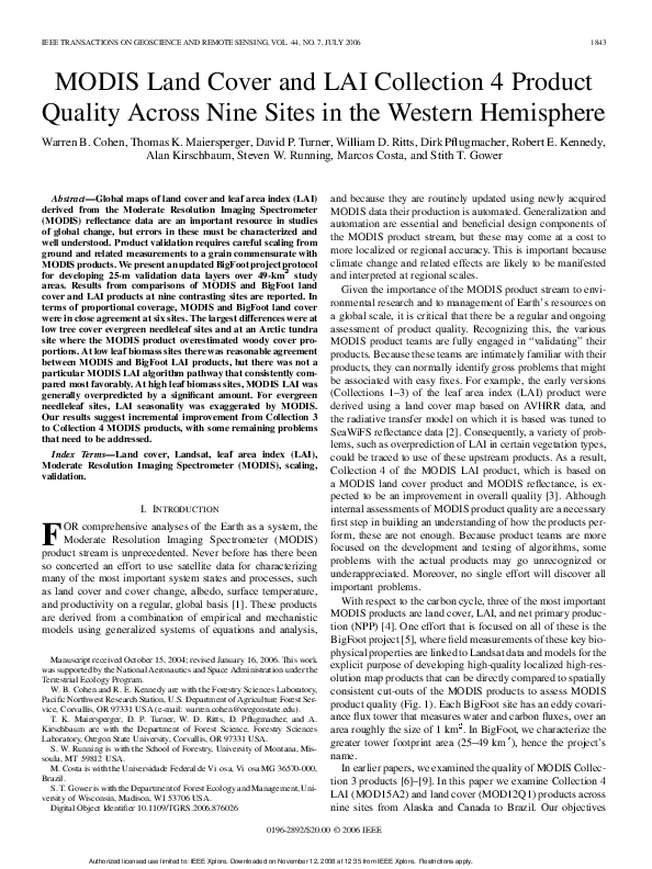With respect to the carbon cycle, three of the most important MODIS products are land cover, LAI, and net primary production (NPP) [4]. One effort that is focused on all of these is the BigFoot project [5], where field measurements of these key biophysical properties are linked to Landsat data and models for the explicit purpose of developing high-quality localized high-resolution map products that can be directly compared to spatially consistent cut-outs of the MODIS products to assess MODIS product quality (Fig. 1). Each BigFoot site has an eddy covariance flux tower that measures water and carbon fluxes, over an area roughly the size of 1 km . In BigFoot, we characterize the greater tower footprint area (25–49 km ), hence the project’s name. In earlier papers, we examined the quality of MODIS Collection 3 products [6]–[9]. In this paper we examine Collection 4 LAI (MOD15A2) and land cover (MOD12Q1) products across nine sites from Alaska and Canada to Brazil. Our objectives 0196-2892/$20.00 © 2006 IEEE Authorized licensed use limited to: IEEE Xplore. Downloaded on November 12, 2008 at 12:35 from IEEE Xplore. Restrictions apply. 1844 IEEE TRANSACTIONS ON GEOSCIENCE AND REMOTE SENSING, VOL. 44, NO. 7, JULY 2006 Fig. 1. BigFoot project conceptual framework. are to assess the quality of the IGBP version of MODIS land cover, representing the year 2001, and the full temporal series of eight-day composite LAI products from 2000 to 2003 over these nine sites. A companion paper by Turner et al. [10] examines the GPP product across three BigFoot sites. TABLE I SITE INFORMATION II. METHODS Detail concerning the methods used by BigFoot to assess MODIS land cover and LAI product quality has been presented elsewhere [6], [11]. Here we only present new detail when relevant. A. Study Sites The nine sites used in this study (Table I) include the four sites from our earlier paper [6] and five new sites. The original sites, described more fully in [6], are Northern Old Black Spruce (NOBS), Harvard Forest (HARV), Konza Prairie (KONZ), and an agricultural system in Illinois (AGRO). The five new sites include: SEVI, the Sevilleta National Wildlife refuge in central New Mexico [12]; TUND, an arctic tundra located near Barrow, Alaska on the Arctic Coastal Plain [13]; TAPA, the Primary Forest Tower Site in the Tapajós National Forest, which is part of the Large Scale Biosphere-Atmosphere Experiment in Amazonia (LBA) [14]; CHEQ, the tall tower site of the Chequamegon Ecosystem-Atmosphere Study (ChEAS) [15]; and METL, the Metolius tower site in Oregon that is part of the Terrestrial Ecosystem Research and Regional Analysis Project [16], [17]. SEVI is a desert grassland consisting largely of perennial bunchgrasses, with small amounts of cacti and shrubs. The site is not grazed by cattle, but is frequently burned. Authorized licensed use limited to: IEEE Xplore. Downloaded on November 12, 2008 at 12:35 from IEEE Xplore. Restrictions apply. COHEN et al.: MODIS LAND COVER AND LAI COLLECTION 4 PRODUCT QUALITY TABLE II LAI FIELD MEASUREMENT INFORMATION 1845 TABLE III LANDSAT ETM+ DATA USED TO MAP LAND COVER AND LAI TUND is low-stature coastal tundra vegetation with large areas of wetland and open water. CHEQ consists of mixed northern hardwoods, aspen, lowlands, and wetlands. Much of the area was logged about 100 years ago, but has since been reforested. METL is a temperate coniferous forest site with areas of grassland and shrubland. Portions of this site have been disturbed by harvesting and wildfire. TAPA is a moist tropical forest consisting largely of evergreen broadleaf species. The site is relatively undisturbed except by natural gap forming processes. Topographic variability is negligible at all sites except KONZ and HARV. B. Field Sampling Design and Measurements At seven of the nine sites, we established 100 plots, each 25 m 25 m, distributed around a square 25-km area where LAI and related data were collected (Table II). At METL [17] and CHEQ [15] there were current, existing LAI measurements collected for other research projects that were available for use. In all cases except TAPA, all plot locations were determined using a real-time differential GPS, with an accuracy of 0.5 m. Although 100 plots were established at TAPA, the spatial accuracy was inadequate for all but ten due to the difficulty of using a GPS under these dense canopies. Because our plot size was close to the resolution of a single Landsat pixel, which was roughly equivalent to tree canopy and gap size at this site, the penalty for inaccurate coregistration of plots and Landsat imagery was high. Thus, only those ten plots were used to model LAI. However, the mean LAI of 5.6 was relatively stable across the 100 plots sd (Table II), such that, although not an ideal situation, the ten plots used were sufficiently representative of the conditions over the full site. For some sites, plots were measured multiple times. The sample design used at the original four sites and at CHEQ was a nested spatial series [15], [18]. That sampling scheme was revised for the other four sites, as reported by Kennedy et al. [19]. At each plot, a set of biophysical measurements was made [20]. Of these, only LAI is reported in this paper. At all but METL, LAI was measured at five subplots, and measurements were averaged to provide a single value for each 25 m 25 m plot. At METL, plot size was 1 ha, and data along a transect within each plot were averaged to calculate a mean value for each plot. Sampling at a given site varied by date, and methods used varied by vegetation type (Table II), as described by Campbell et al. [20]. At METL, LAI was measured optically with an LAI-2000, as described by Law et al. [17]. See Gower et al. [21] for a discussion of common assumptions and errors in measurements of LAI. Land cover was observed using a number of methods, depending on site and data availability. At all sites, IGBP land cover classes [6] were observed at each of the plots. This dataset was augmented by interpretation of contemporaneous high-resolution traditional and digital airphotos and IKONOS imagery. At NOBS, in addition to these observations, percent tree cover was measured at nine systematically spaced subplots over the 100 plots using an upward-looking digital camera, as described by Cohen et al. [11]. This enabled direct measurement of tree cover percent. At the other sites, percent tree and woody cover was quantified from the photo and IKONOS data [6]. C. Landsat Data 1) Preprocessing: Landsat Enhanced Thematic Mapper Plus (ETM+) imagery was used at each site to develop land cover and LAI maps, with most maps based on multiple image dates (Table III). All imagery was acquired at level 1G processing,1 with a cell size of 30 m, and UTM (WGS84) projection. At seven sites (all except NOBS and TAPA), U.S. Geological Survey digital orthophoto quadrangles were used 1http://ltpwww.gsfc.nasa.gov/IAS/handbook/handbook_toc.html Authorized licensed use limited to: IEEE Xplore. Downloaded on November 12, 2008 at 12:35 from IEEE Xplore. Restrictions apply. 1846 IEEE TRANSACTIONS ON GEOSCIENCE AND REMOTE SENSING, VOL. 44, NO. 7, JULY 2006 for georeferening the Landsat data. At NOBS and TAPA, a panchromatic IKONOS image was used after it was registered to the Earth’s surface using several global positioning system (GPS) points collected in the field. All Landsat images were resampled to 25-m resolution, with 10 m RMSE. The COST absolute radiometric correction model of Chavez [22] was applied to each image to convert digital counts to reflectance, as given in [6]. All ETM+ images were translated into tasseled cap brightness, greenness, and wetness using the Thematic Mapper (TM) reflectance factor coefficients [23], after they were atmospherically corrected and radiometrically normalized using pseudoinvariant features [11]. 2) Mapping: At each site, BigFoot measurements and error assessments were conducted on the core 25-km area that defined the site around the flux tower. However, by mapping land cover and LAI over an area that included a 1-km buffer around the core site, we increased the number of potential MODIS cells we could use for comparison with BigFoot maps from 25 to 49. We felt that this modest extension of area beyond where measurements were made was reasonable, as these sites are generally representative of their local biophysical environments. To check the validity of this assumption, we visited every site and its immediate environment and determined that there was no substantive change in vegetation properties in the buffer relative to the core site. Additionally, we examined the reflectance properties of the images used, and these were consistent within and without the buffer. a) Land cover: BigFoot land cover maps were based on the IGBP variant of MODIS land cover products, which has 17 cover classes [6]. Where relevant, the maps were based on the multidate stack of ETM+ band data or tasseled cap indexes at each site (Table III). The goal was to map land cover at the peak of the growing season for the year represented. Details of the approach for mapping land cover and assessing accuracy of land cover at BigFoot sites are given in [6]. We compared 25-m distributions of BigFoot land cover against 1-km MODIS distributions. b) LAI: As described in [6] and [11], regression analysis was used to model the relationship between spectral data and LAI at each site. To the extent possible, we developed separate models for each major vegetation cover class or class group. To map LAI across a study site, the model developed for a given class at a given site was applied to those pixels labeled as that class in the land cover map. Some vegetation classes existed as small, scattered patches at a given site, e.g., the grassland class at AGRO. As we did not sample those classes in the field, we synthesized LAI values from the literature, as follows: water, barren, urban/built were assigned a value of 0.0; grassland and permanent wetland were assigned 1.0; savanna was assigned 1.5; woody savanna was assigned 2.0; and cropland and deciduous broadleaf forest were assigned 3.0 and 5.0, respectively. To assess errors in the LAI maps, we used the cross-validation procedure [11]. Additionally, predicted versus observed plots were developed, and overall bias and variance ratios were calculated. Bias was calculated as the mean of the predicted values minus the mean of the observed values, such that a positive bias equated to a mean overprediction, and vice versa. Variance ratio was calculated as the standard deviation of the predicted values divided by the standard deviation of the observed values. As such, a ratio of greater than one meant that the prediction standard deviation was greater than the observed standard deviation, and vice versa. In general, the date represented by each map was the field measurement date. However, at the coniferous forested sites (i.e., METL and NOBS), we assumed LAI values were relatively stable throughout the growing season and across years. As such, at these sites and at TPA our mapped dates represent the acquisition date of the Landsat image used, or the one that was closest to the middle of the growing season if more than one image was used. For some sites without remeasurement dates, we updated the land cover maps for subsequent years using change detection techniques with new Landsat images, and then applied our existing LAI spectral models, as described by Cohen et al. [6]. We realize that LAI values exhibit potentially important temporal variability that we did not account for and that one should account for this variability whenever possible. 3) BigFoot-MODIS Comparisons: MODIS Collection 4 products were in the sinusoidal projection and BigFoot products were in UTM WGS84. To compare these, BigFoot maps were reprojected into sinusoidal projection, permitting direct overlay and comparison of land cover and LAI data products at the site level [6]. Only those MODIS cells completely filled with mapped Landsat pixels were used for comparison, with the maximum potential number being 49. At each site, we summarized both sets of maps to characterize proportions of land cover classes as frequency histograms in each dataset. For LAI we plotted the mean and standard deviation of 1-km MODIS LAI eight-day composite data for the years 2000 to 2003. On the same graphs, mean and standard deviation of the 25-m resolution BigFoot ETM+ surfaces were plotted. The MODIS LAI algorithm has multiple pathways, including the main and the backup [24]. The main (or default) algorithm pathway is based on a radiative transfer model that expects certain conditions to be met in the input variables (e.g., reflectance, land cover). When these conditions are not met, the backup (or empirical) algorithm pathway may be used. Also, if input reflectance does not meet certain threshold conditions, it may be identified as in the “saturation domain,” in which case the estimate of LAI produced is considered of suspect quality. There are also several other conditions that lead to a variety of certainty (or quality) levels associated with individual estimates. As such, every MODIS LAI estimate has quality flags that describe certain characteristics of the input data and thus the quality of the LAI prediction. For our analysis, we have stratified the MODIS estimates into four categories, based on quality flag information provided with each estimate. The usable main RT category includes only those estimates that are “OK” or “best” where the main algorithm was used in a nonsaturated condition. Usable main RT with saturation is the same, but under saturation conditions. The usable empirical category includes OK and best combined, but where the empirical algorithm was used to produce the estimate. Not usable includes estimates that were not flagged as OK or best or where clouds were present or other problems were identified. To enhance our understanding of the behavior of the MODIS algorithm, we examined the usage of these categories for an area of 100 km 100 km around each study site. Authorized licensed use limited to: IEEE Xplore. Downloaded on November 12, 2008 at 12:35 from IEEE Xplore. Restrictions apply. COHEN et al.: MODIS LAND COVER AND LAI COLLECTION 4 PRODUCT QUALITY 1847 Fig. 2. BigFoot land cover (top) and LAI (bottom) maps, and IKONOS and ADAR false-color images (middle), of the nine study sites. Of the 17 IGBP classes, a total of 14 were mapped at the sites. III. RESULTS A. BigFoot Surfaces 1) Land Cover: Land cover maps of the nine sites indicate that, across sites, 14 of the 17 MODIS IGBP land cover classes were evaluated (Fig. 2). Overall, errors rates were low ( 11%) (Table IV), with site level errors varying between 2% and 19% depending on vegetation complexity. Comparing the patterns of land cover with patterns of reflectance in high-resolution images of the sites (Fig. 2), provides additional confidence that Authorized licensed use limited to: IEEE Xplore. Downloaded on November 12, 2008 at 12:35 from IEEE Xplore. Restrictions apply. 1848 IEEE TRANSACTIONS ON GEOSCIENCE AND REMOTE SENSING, VOL. 44, NO. 7, JULY 2006 TABLE IV SITE-SPECIFIC ERROR MATRIX FOR BIGFOOT LAND COVER MAPS. GIVEN ARE NUMBERS OF OBSERVATIONS BY SITE AND COVER CLASS TABLE V RESULTS OF LAI MODEL CROSS-VALIDATION Fig. 3. Observed versus predicted for the BigFoot LAI maps at the nine study sites, from cross-validation. the BigFoot cover maps closely follow actual land cover pattern at the sites. For example, at METL, the denser vegetation is mapped as closed forest ( 60% tree cover), whereas more open forest conditions ( 60% tree cover) are mapped as woody savanna (30% to 60% tree cover) and savanna (10% to 30% Authorized licensed use limited to: IEEE Xplore. Downloaded on November 12, 2008 at 12:35 from IEEE Xplore. Restrictions apply. COHEN et al.: MODIS LAND COVER AND LAI COLLECTION 4 PRODUCT QUALITY Fig. 4. Proportions of IGBP classes in the BigFoot and MODIS land cover maps of the nine study sites. Authorized licensed use limited to: IEEE Xplore. Downloaded on November 12, 2008 at 12:35 from IEEE Xplore. Restrictions apply. 1849 1850 IEEE TRANSACTIONS ON GEOSCIENCE AND REMOTE SENSING, VOL. 44, NO. 7, JULY 2006 tree cover). Note also that NOBS (particularly in the northern four-fifths of the site) consists largely of woody savanna and savanna and very little evergreen needleleaf forest. In addition to matching the spectral patterns in the reflectance values the BigFoot land cover maps also matched what we saw during field visits. Spatial patterns across the sites were highly variable. The simplest were TAPA, SEVI, and AGRO (if soybeans and corn are collapsed to cropland), each consisting largely of one class. The most complex were the boreal and subboreal forest sites NOBS and CHEQ. Small patches ( 1 km) should not resolve in MODIS 1-km maps. This is particularly so for NOBS, CHEQ, HARV, TUND, and KONZ. Forested sites containing small patches of one type as part of a matrix of another type should increase the amount the mixed forest type at the expense of the more spatially detailed types. CHEQ, for example, had very few 1-km or larger patches of evergreen needleleaf, embedded largely in a matrix of deciduous broadleaf. As such, the amount of mixed forest at 1 km is likely to be significantly larger than that type at the grain Landsat ( 30 m). 2) LAI: Landsat-based LAI maps of the sites indicate a high correspondence among land cover, reflectance, and LAI patterns (Fig. 2). The lowest LAIs were found at two of the grassland sites (TUND and SEVI) and the highest LAIs were observed at closed forest sites, particularly TAPA and HARV. Errors in predicted LAI overall (Fig. 3 and Table V) were relatively low (e.g., RMSE of 0.73, with RMSE 6% of the range of predictions). Among sites, RMSEs varied from 0.03 at SEVI to 1.47 at CHEQ. B. BigFoot-MODIS Comparisons 1) Land Cover: TAPA, AGRO, and SEVI had the least spatial complexity of IGBP vegetation classes among the sites. The mapped proportions of cover classes at these sites were essentially identical (TAPA and SEVI) or nearly so (AGRO) for BigFoot and MODIS (Fig. 4). MODIS mapped KONZ as nearly pure grassland, which was expected given the fine-grained nature of patches of other vegetation classes. MODIS labeled much of the TUND site as open shrubland, whereas BigFoot observed (in the field and via Landsat) mostly grassland. The difference between grassland and open shrubland can be minimal, as, using the IGBP system, the site could consist of 90% grassland and 10% shrubland, but be still be labeled as shrubland. The North American forest sites were spatially complex. HARV included several small evergreen needleleaf forest patches and other classes that were unresolvable in the MODIS land cover product. As a result, this site appeared to MODIS as a deciduous broadleaf and mixed forest site, which at 1-km grain it is. The best example of fine-grained patches not being resolved in the MODIS product was CHEQ, within which it had been mapped as a largely mixed forest. Again, this is correct at 1-km grain size, because this site consists largely of numerous, well-distributed sub-MODIS pixel size patches of ENF and DBF. METL and NOBS were mapped largely as woody savanna and related classes by BigFoot, but as evergreen needleleaf forests in the MODIS product. Although these are colloquially thought of as evergreen needleleaf forest sites, they consisted mostly of forests that were less than 60% tree cover, and hence are by IGBP definition not evergreen needleleaf forest sites. Rather, in IGBP terms, they tend more toward being savanna and woody savanna sites. 2) LAI: The MODIS LAI product can be complex to interpret. One reason is that LAI estimates differ depending on algorithm pathway used. Focusing first on the pathway used over the 100 km 100 km greater site area, we observed considerable variability in pathway used over the course of the year (Fig. 5). SEVI was the simplest site in this regard, with nearly 100% of the LAI values assigned by the main algorithm under ideal or near ideal conditions. The same was true for KONZ and AGRO; however, at AGRO the dominant algorithm pathway was empirical during the peak of the growing season. At HARV and CHEQ the empirical algorithm pathway also dominated during the growing season. Although at METL and NOBS there was significant usage of the empirical pathway, during the growing season the main algorithm was used predominantly. TAPA and TUND are relatively cloudy sites, such that much of the time during a year MODIS data were unusable for LAI mapping within eight-day intervals. At these sites, although there was significant use of the empirical pathway, during the growing season the proportion of main algorithm usage increased. No MODIS data existed for TUND prior to 2002. Over the local site area (up to 49 km ), direct comparisons of MODIS and BigFoot LAI maps enable an assessment of MODIS LAI quality in relation to algorithm pathway (Fig. 6). In both datasets, the desert grassland (SEVI) and Arctic tundra (TUND) sites had the lowest LAIs. At SEVI, the main algorithm pathway was used almost exclusively. At this site, precipitation was much higher in 2002 than in 2003 and both datasets showed a correspondingly higher LAI in 2002; see also [10]. At TUND there was only one BigFoot observation date, but the mean LAI predicted at that date by MODIS used the main algorithm and was nearly equal to that of BigFoot. KONZ is interesting in that, at the local level the empirical algorithm pathway dominated during the growing season, in contrast to use of the main pathway dominating over the greater 100 km 100 km area. Overall, the mean LAI values for KONZ in the MODIS datasets were similar to those of the BigFoot datasets. However, the seasonal dynamics for these two datasets appeared somewhat different, and the algorithm pathway that provided estimates that most closely matched those of BigFoot’s was not consistent. Additionally at this site, mean LAI across algorithm pathways near the peak of the growing season was higher than BigFoot mean LAI by as much as 2.0. At AGRO, for the one year that common datasets existed, it appears that the mean in both datasets was similar at two times during the growing season. However at both KONZ and AGRO, because multiple algorithm pathways were used locally during the growing, we can begin to see differences in pathway estimates. At these sites, there appeared to be a strong stratification of estimated values, with the main algorithm without saturation providing the lowest estimates and the main algorithm with saturation providing the highest. Empirical estimates were intermediate. At HARV and CHEQ, stratification of estimate value by pathway was more clearly evident. At both of these sites the main algorithm without saturation provided estimates that were closest to BigFoot estimates, but those estimates were not stable Authorized licensed use limited to: IEEE Xplore. Downloaded on November 12, 2008 at 12:35 from IEEE Xplore. Restrictions apply. COHEN et al.: MODIS LAND COVER AND LAI COLLECTION 4 PRODUCT QUALITY 1851 over time. The mean across pathway estimates for these sites during the growing season were between 2 and 3 higher than those estimated by BigFoot. At METL seasonal LAI values should be relatively stable, varying at most by 30% of maximum (derived from [16] and [25]). This suggests that the seasonal dynamics of the MODIS product, which varied from roughly 1 to 4, was unrealistic at this site. Interestingly, at this site, the empirical and saturation algorithm pathways provided the lowest estimated values. At NOBS, although seasonal dynamics of LAI exist, these are mostly associated with the understory, which in this system is commonly a small proportion of total LAI [26]. Consequently, the variation observed in the MODIS LAI product (0 to 5) is highly unrealistic. Moreover, like at METL, the mean product estimate at NOBS was unstable during its growing season trajectory, bouncing from a value of 2 to 5, for example, in neighboring date bins. Additionally, the mean value for this site was higher than that observed by BigFoot by as much as 2 during peak growing season. The MODIS LAI product for TAPA was very unstable, with the mean generally varying between 3 and 6. The mean BigFoot estimates for that site was around 6, which was most closely approximated by the saturation pathway. exists across these two sites. At SEVI and TAPA, which are both essentially single class sites, Collection 4 MODIS land cover corresponded closely to BigFoot land cover. TUND is an Arctic grassland, but was labeled by MODIS as an open shrubland. Shrubs are known to more readily inhabit Arctic grasslands further inland, but at this coastal site there was almost a total absence of shrubs. No land cover classification system suits all needs [27]. The MODIS IGBP classification system, although quite useful and generally accepted by the science community, may not be the best system to use for MODIS products, particularly if it continues to contain ambiguities in definitions of classes, as described by Cohen et al. [6]. Also, like most classification systems it is relatively inflexible. A trend toward continuous fields/estimates [28], [29] is a viable solution to the general inflexibility of class definitions. Also, it may be necessary to consider a flexible system based on local characteristics. For example, if the common reference to treed boreal ecosystems is to call them forests, then the classification system should allow for that, even though they may not contain tree covers in excess of 60%. IV. DISCUSSION AND CONCLUSION When designing an LAI algorithm based on MODIS data to produce an ongoing series of global LAI maps for use in regional to global Earth-system process models, several criteria are vitally important. Primary among these are that the algorithm produce maps that are accurate at the biome or regional level, and that it correctly respond to biome-level LAI trajectories associated with interannual climate variability. The algorithm should also be sensitive to meaningful perturbations to LAI, such as from significant disturbances. Although the MODIS LAI Collection 4 product is an improvement toward these goals over the Collection 3 product, our results indicate that there are still significant problems to be addressed. These include overprediction of LAI in forested biomes, instability of LAI trajectories during the growing season that are not related to vegetation change, and unrealistic dormant-season LAI in evergreen needleleaf forest sites. Given these findings, it is important to consider the results of similar studies to facilitate a more general understanding of MODIS LAI product quality. In a global assessment of MODIS LAI predictions, the best retrievals were found to be from the main algorithm without saturation [3]. This was consistent with our findings at all but TAPA, and to a lesser degree at KONZ, AGRO, and possibly METL. Confirming what we found in this study, low LAI sites (especially those in arid and semiarid regions below an LAI of about 2) were found to be correctly mapped by MODIS [2], [30], [31]. At KONZ, Huang et al. [32] confirmed our observations for Collection 3 data of disagreement with field measurements, differences between main and backup estimates, and low usage of the main algorithm [6]. Over the greater AGRO area of largely broadleaf crops, Tan et al. [2] confirmed our earlier findings for Collection 3 data that usage of the empirical algorithm pathway dominated and that there were substantive overestimations of peak summer LAI values. Consistent with our findings, Leuning et al. [33] and Fang and Liang [34] observed significant overpredictions by the Collection 4 LAI product at forested sites. For validation of MODIS land cover and LAI, the BigFoot strategy used observations from field measurements and high-resolution image data (e.g., IKONOS) to train statistical models based primarily on Landsat ETM+ data. The results of this strategy at a given site were high-quality map representations of vegetation characteristics, lending validity to their use as a reference against which to compare MODIS land products. Following is a synthesis of observations from this study, and where relevant these observations are given in the context of related studies. A. MODIS Land Cover Considering the inherent limitations of a 1-km dataset and use of a less than ideal classification system, results of this study indicate that the MODIS land cover product is generally accurate across a large assortment of biomes and cover types. We know for land cover that the 1-km MODIS product cannot resolve small patches of vegetation that do not dominate a pixel. Given that limitation, we noted in our earlier validation study that, at the site level, the MODIS Collection 3 land cover product was in close correspondence with actual land cover as depicted by BigFoot at HARV, KONZ, and AGRO [6]. The same was true here for Collection 4 data, and for CHEQ. At NOBS, we found that the earlier MODIS product labeled the site primarily as an evergreen needleleaf forest, whereas BigFoot found the site to be a mix of open shrubland, savanna, and woody savanna. In the Collection 4 product, we noted here the same inconsistency at this site. A similar problem was noted at METL, another relatively open evergreen needleleaf forest site. In both cases, the problem seems to be one of strict definition versus colloquialism, as the MODIS IGBP evergreen needleleaf forest class requires the presence of greater than 60% tree cover. Our observations indicate a significantly lower canopy cover generally B. MODIS LAI Authorized licensed use limited to: IEEE Xplore. Downloaded on November 12, 2008 at 12:35 from IEEE Xplore. Restrictions apply. 1852 Fig. 5. IEEE TRANSACTIONS ON GEOSCIENCE AND REMOTE SENSING, VOL. 44, NO. 7, JULY 2006 Relative frequency of MODIS LAI algorithm pathway usage between 2000 and 2003 for 100 km We did not explicitly examine the accuracy of MODIS LAI seasonal trajectories. However, others have and the results are mixed. Privette et al. [30] found that MODIS LAI seasonality in arid and semiarid, low LAI systems follows independent observations. However, early onset of increase in LAI with new growth has been observed elsewhere in a similar system [31]. Acceptable representation by the MODIS LAI product of LAI seasonality has also been noted in temperate mixed forest [35]. But like we found at NOBS, Yang et al. [3] identified spurious 2 100 km areas around the nine study sites. seasonality in high-latitude forests. They attributed this to use of the backup algorithm, whereas at our site the main algorithm pathway dominated through the growing season. Tian et al. [36] similarly noted that winter retrievals for evergreen forests in northern latitudes were significantly underestimated by the Collection 4 product. Huang et al. [32] state that the LAI algorithm anomalies noted in the greater KONZ area are resolved and no longer a problem for the Collection 4 algorithm. Although for the greater land- Authorized licensed use limited to: IEEE Xplore. Downloaded on November 12, 2008 at 12:35 from IEEE Xplore. Restrictions apply. COHEN et al.: MODIS LAND COVER AND LAI COLLECTION 4 PRODUCT QUALITY 1853 Fig. 5. (Continued). Relative frequency of MODIS LAI algorithm pathway usage between 2000 and 2003 for 100 km scape around KONZ, there is a definite and substantive increase in the use of the main algorithm, much of that landscape is dif- 2 100 km areas around the nine study sites. ferent from the grassland preserve itself. Additionally, for that area we found that the backup algorithm was used predomi- Authorized licensed use limited to: IEEE Xplore. Downloaded on November 12, 2008 at 12:35 from IEEE Xplore. Restrictions apply. 1854 IEEE TRANSACTIONS ON GEOSCIENCE AND REMOTE SENSING, VOL. 44, NO. 7, JULY 2006 Fig. 6. MODIS LAI estimates by algorithm pathway and across pathways between 2000 and 2003 for the 7 km a description of why BigFoot LAI values in this figure and Table II are different. nantly during the growing season, and that for the grassland area itself, the backup algorithm may more accurately estimate LAI during the peak of the growing season. This may have, as of yet, unknown implications for vast areas of grassland around the globe. For the greater AGRO area, Tan et al. [2] claim that the problems identified in Collection 3 have been addressed and that there is now a better fit of the MODIS predictions with observations by BigFoot. Our results suggest that Collection 4 esti- 2 7 km areas of the nine study sites. See [6] for mate quality around the AGRO site is definitely improved relative to Collection 3, but that peak growing season estimates are still derived from the empirical backup algorithm, not the main algorithm. Tan et al. [2] state that estimates from the backup algorithm should be used with extreme caution, and as demonstrated in this study, algorithm pathway can have a profound impact on the quality of the MODIS LAI product. Thus, the product user must pay close attention to the quality flags associated with the Authorized licensed use limited to: IEEE Xplore. Downloaded on November 12, 2008 at 12:35 from IEEE Xplore. Restrictions apply. COHEN et al.: MODIS LAND COVER AND LAI COLLECTION 4 PRODUCT QUALITY Fig. 6. (Continued). MODIS LAI estimates by algorithm pathway and across pathways between 2000 and 2003 for the 7 km See [6] for a description of why BigFoot LAI values in this figure and Table II are different. Authorized licensed use limited to: IEEE Xplore. Downloaded on November 12, 2008 at 12:35 from IEEE Xplore. Restrictions apply. 1855 2 7 km areas of the nine study sites. 1856 IEEE TRANSACTIONS ON GEOSCIENCE AND REMOTE SENSING, VOL. 44, NO. 7, JULY 2006 specific dataset they are using. Moreover, users of the current MODIS LAI product need to understand that they cannot use the data without careful consideration of product quality and implications of inaccuracies in the product for their models. Ideally, the main algorithm pathway should be used most of the time when estimating LAI within a given region or biome. In a study by Yang et al. [3], it was found globally that the main algorithm was used 50% of the time for the Collection 3 product, but that for Collection 4 the main algorithm was used 70% of the time. This improvement globally is important, but our results indicate that, on a more regional level, there may still be problems. For four of the nine BigFoot sites (HARV, CHEQ, TAPA, and AGRO), the backup algorithm was used at least 50% of the time during much of the growing season, and nearly exclusively at TUND and NOBS during the dormant season. MODIS LAI and fPAR products are very closely related [22]. As both of these are used in the MODIS GPP/NPP algorithm [37], the errors in the LAI and fPAR estimates may propagate into the GPP and NPP products. Turner et al. [10] discuss this more thoroughly. LAI products from MODIS and other satellite-borne sensors are also intended for use in initializing LAI in the atmosphere–biosphere exchange component of general circulation models [38]. In that case, errors in the MODIS LAI products would potentially propagate into the water and energy balance of the climate model. Also, satellite-based LAI products have potential for use in validating the LAI outputs in prognostic carbon cycle models, i.e., those that generate their own LAI based on local climate and soil properties [39]. Uncertainty in the MODIS LAI products would limit the degree to which they could serve as reference values. ACKNOWLEDGMENT The authors greatly thank the numerous people who helped make the BigFoot project a success, and the reviewers of this paper for their contributions to its presentation. REFERENCES [1] C. O. Justice, J. R. G. Townshend, E. F. Vermote, E. Masouka, R. E. Wolfe, N. Saleous, D. P. Roy, and J. T. Morisette, “An overview of MODIS Land data processing and product status,” Remote Sens. Environ., vol. 83, pp. 3–15, 2002. [2] B. Tan, D. Huang, J. Hu, W. Yang, P. Zhang, N. V. Shabanov, Y. Knyazikhin, R. R. Nemani, and R. B. Myneni, “Assessment of the broadleaf crops leaf area index product from the Terra MODIS instrument,” Agricult. Forest Meteorol., vol. 135, pp. 124–134, 2005. [3] W. Yang, D. Huang, B. Tan, J. C. Stroeve, N. V. Shabanov, Y. Knyazikhin, R. R. Nemani, and R. B. Myneni, “Analysis of leaf area index and fraction of PAR absorbed by vegetation products from the Terra MODIS sensor: 2000–2005,” IEEE Trans. Geosci. Remote Sens., vol. 44, no. 7, pp. 1829–1842, Jul. 2006. [4] D. P. Turner, S. V. Ollinger, and J. S. Kimball, “Integrating remote sensing and ecosystem process models for landscape- to regional-scale analysis of the carbon cycle,” BioScience, vol. 54, pp. 573–584, 2004. [5] W. B. Cohen and C. O. Justice, “Validating MODIS terrestrial ecology products: Linking in situ and satellite measurements,” Remote Sens. Environ., vol. 70, pp. 1–3, 1999. [6] W. B. Cohen, T. K. Maiersperger, Z. Yang, S. T. Gower, D. P. Turner, W. D. Ritts, M. Berterretche, and S. W. Running, “Comparisons of land cover and LAI estimates derived from ETM+ and MODIS for four sites in North America: A quality assessment of 2000/2001 provisional MODIS products,” Remote Sens. Environ., vol. 88, pp. 233–255, 2003. [7] D. P. Turner, W. D. Ritts, W. B. Cohen, S. T. Gower, M. Zhao, S. W. Running, S. C. Wofsy, S. Urbanski, A. L. Dunn, and J. W. Munger, “Scaling gross primary production (GPP) over boreal and deciduous forest landscapes in support of MODIS GPP validation,” Remote Sens. Environ., vol. 88, pp. 256–270, 2003. [8] D. P. Turner, S. Urbanski, D. Bremer, S. C. Wofsy, T. Meyers, S. T. Gower, and M. Gregory, “A cross-biome comparison of daily light use efficiency for gross primary production,” Glob. Change Biol., vol. 9, pp. 383–395, 2003. [9] D. P. Turner, W. Ritts, W. B. Cohen, T. Maiersperger, S. T. Gower, A. Kirschbaum, S. W. Running, M. Zhao, S. Wofsy, A. Dunn, B. Law, J. Campbell, W. Oechel, H. J. Kwon, T. Meyers, E. Small, S. Kurc, and J. Gamon, “Site-level evaluation of satellite-based global GPP and NPP monitoring,” Glob. Change Biol., vol. 11, pp. 1–19, 2005. [10] D. P. Turner, W. D. Ritts, M. Zhao, S. A. Kurc, A. L. Dunn, S. C. Wofsy, E. E. Small, and S. W. Running, “Assessing interannual variation in MODIS-based estimates of gross primary production,” IEEE Trans. Geosci. Remote Sens., vol. 44, no. 7, pp. 1899–1907, Jul. 2006. [11] W. B. Cohen, T. K. Maiersperger, S. T. Gower, and D. P. Turner, “An improved strategy for regression of biophysical variables and Landsat ETM+ data,” Remote Sens. Environ., vol. 84, pp. 561–571, 2003. [12] R. J. Gosz and J. R. Gosz, “Species interactions on the biome transition zone in New Mexico: Response of blue grama (Bouteloua gracilis) and black grama (Bouteloua eripoda) to fire and herbivory,” J. Arid Environ., vol. 34, pp. 101–114, 1996. [13] Y. Harazono, M. Mano, A. Miyata, R. C. Zulueta, and W. C. Oechel, “Inter-annual carbon dioxide uptake of a wet sedge tundra ecosystem in the Arctic,” Tellus, vol. 55, pp. 215–231, 2003. [14] M. Keller, A. Alencar, G. P. Asner, B. Braswell, M. Bustamante, E. Davidson, T. Feldpausch, E. Fernandes, M. Goulden, P. Kabat, B. Kruijt, F. Luizao, S. Miller, D. Markewitz, A. D. Nobre, C. A. Nobre, N. P. Filho, H. da Rocha, P. S. Dias, C. von Randow, and G. L. Vourlitis, “Ecological research in the large-scale biosphere–atmosphere experiment in amazonia: Early results,” Ecol. Appl., vol. 14, pp. S3–S16, 2004. [15] S. N. Burrows, S. T. Gower, M. K. Clayton, D. S. Mackay, D. E. Ahl, J. M. Norman, and G. Diak, “Application of geostatistics to characterize leaf area index (LAI) from flux tower to landscape scales using a cyclic sampling design,” Ecosystems, vol. 5, pp. 667–679, 2002. [16] B. E. Law, S. Van Tuyl, A. Cescatti, and D. D. Baldocchi, “Estimation of leaf area index in open-canopy ponderosa pine forests at different successional stages and management regimes in Oregon,” Agricult. Forest Meteorol., vol. 108, pp. 1–14, 2001. [17] B. E. Law, D. Turner, J. Campbell, O. J. Sun, S. Van Tuyl, W. D. Ritts, and W. B. Cohen, “Disturbance and climate effects on carbon stocks and fluxes across western Oregon USA,” Glob. Change Biol., vol. 10, pp. 1429–1444, 2004. [18] M. Berterretche, A. T. Hudak, W. B. Cohen, T. K. Maiersperger, S. T. Gower, and J. Dungan, “Comparison of regression and geostatistical methods for mapping leaf area index (LAI) with Landsat ETM+ data over a boreal forest,” Remote Sens. Environ., vol. 96, pp. 49–61. [19] R. E. Kennedy, W. B. Cohen, D. Oetter, C. Cooper, A. A. Kirschbaum, T. K. Maiersperger, and S. T. Gower, “Constrained stochastic sampling for spatial studies in ecology,” Remote Sens. Environ., submitted for publication. [20] J. L. Campbell, S. Burrows, S. T. Gower, and W. B. Cohen, “BigFoot: Characterizing Land Cover, LAI, and NPP at the Landscape Scale for EOS/MODIS Validation. Field Manual 2.1.,” Oak Ridge Nat. Lab., Oak Ridge, TN, Environ. Sci. Div. Pub. 4937, 1999. [21] S. T. Gower, C. J. Kucharik, and J. M. Norman, “Direct and indirect estimation of leaf area index, fAPAR, and net primary production of terrestrial ecosystems,” Remote Sens. Environ., vol. 70, pp. 29–51, 1999. [22] P. S. Chavez, Jr., “Image-based atmospheric corrections—revisited and improved,” Photogramm. Eng. Remote Sens., vol. 62, pp. 1025–1036, 1996. [23] E. P. Crist, “A TM tasseled cap equivalent transformation for reflectance factor data,” Remote Sens. Environ., vol. 17, pp. 301–306, 1985. [24] R. B. Myneni, S. Hoffman, Y. Knyazikhin, J. L. Privette, J. Glassy, Y. Tian, Y. Wang, X. Song, Y. Zhang, G. R. Smith, A. Lotsch, M. Friedl, J. T. Morisette, P. Votava, R. R. Nemani, and S. W. Running, “Global products of vegetation leaf area and fraction absorbed PAR from one year of MODIS data,” Remote Sens. Environ., vol. 83, pp. 214–231, 2002. [25] B. E. Law, M. G. Ryan, and P. M. Anthoni, “Seasonal and annual respiration of a ponderosa pine ecosystem,” Global Change Biol., vol. 5, pp. 169–182, 1999. [26] S. T. Gower, J. G. Vogel, J. M. Norman, C. J. Kucharik, S. J. Steele, and T. K. Stow, “Carbon distribution and aboveground net primary production in aspen, jack pine, and black spruce stands in Saskatchewan and Manitoba, Canada,” J. Geophys. Res., vol. 102, pp. 29 029–29 041, 1997. Authorized licensed use limited to: IEEE Xplore. Downloaded on November 12, 2008 at 12:35 from IEEE Xplore. Restrictions apply. COHEN et al.: MODIS LAND COVER AND LAI COLLECTION 4 PRODUCT QUALITY 1857 [27] J. R. Thomlinson, P. V. Bolstad, and W. B. Cohen, “Coordinating methodologies for scaling landcover classifications from site-specific to global: Steps toward validating global map products,” Remote Sens. Environ., vol. 70, pp. 16–28, 1999. [28] W. B. Cohen, T. K. Maiersperger, T. A. Spies, and D. R. Oetter, “Modeling forest cover attributes as continuous variables in a regional context with Thematic Mapper data,” Int. J. Remote Sens., vol. 22, pp. 2279–2310, 2001. [29] M. C. Hansen, R. S. DeFries, J. R. G. Townshend, R. Sohlberg, C. Dimiceli, and M. Carroll, “Toward an operational MODIS continuous fields of percent tree cover algorithm: Examples using AVHRR and MODIS data,” Remote Sens. Environ., vol. 83, pp. 303–319, 2002. [30] J. Privette, R. B. Myneni, Y. Knyazikhin, M. Mukelabai, G. Roberts, Y. Tian, Y. Wang, and S. G. Leblanc, “Early spatial and temporal validation of MODIS LAI product in the southern African Kalahari,” Remote Sens. Environ., vol. 83, pp. 232–243, 2002. [31] R. Fensholt, I. Sandholt, and M. S. Rasmussen, “Evaluation of MODIS LAI, fAPAR and the relation between fAPAR and NDVI in a semi-arid environment using in situ measurements,” Remote Sens. Environ., vol. 91, pp. 490–507, 2004. [32] D. Huang, W. Yang, B. Tan, M. Rautiainen, P. Zhang, N. V. Shabanov, S. Linder, Y. Knyazikhin, and R. B. Myneni, “The importance of measurement errors for deriving accurate reference leaf area index maps for validation of moderate-resolution satellite LAI products,” IEEE Trans. Geosci. Remote Sens., vol. 44, no. 7, pp. 1866–1871, Jul. 2006. [33] R. Leuning, H. A. Cleugh, S. J. Zegelin, and D. Hughes, “Carbon and water fluxes over a temperate Eucalyptus forest and tropical wet/dry savanna in Australia: Measurements and comparison with MODIS remote sensing estimates,” Agricult. Forest Meteorol., vol. 129, pp. 153–173, 2005. [34] H. Fang and S. Liang, “A hybrid inversion method for mapping leaf area index from MODIS data: Experiments and application to broadleaf and needleleaf canopies,” Remote Sens. Environ., vol. 94, pp. 405–424, 2005. [35] S. Kang, S. W. Running, J.-H. Lim, M. Zhao, C.-R. Park, and R. Loehman, “A regional phenology model for detecting onset of greenness in temperate mixed forests: An application of MODIS leaf area index,” Remote Sens. Environ., vol. 86, pp. 232–242, 2003. [36] Y. Tian, R. E. Dickenson, L. Zhou, X. Zeng, Y. Dai, R. B. Myneni, Y. Knyazikhin, X. Zhang, M. Freidl, H. Yu, W. Wu, and M. Shaikh, “Comparison of seasonal and spatial variations of leaf area index and fraction of absorbed photosynthetically active radiation from Moderate Resolution Imaging Spectroradiometer (MODIS) and common land model,” J. Geophys. Res., vol. 109, no. D01103, 2004. DOI: 10.1029/2003JD003777. [37] S. W. Running, P. E. Thornton, R. Nemani, and J. M. Glassy, “Global terrestrial gross and net primary productivity from the earth observing system,” in Methods in Ecosystem Science, O. E. Sala, R. B. Jackson, H. A. Mooney, and R. W. Howarth, Eds. New York: Springer-Verlag, pp. 44–57. [38] T. N. Chase, R. A. Pielke, R. Nemani, and S. W. Running, “Sensitivity of a general circulation model to global changes in leaf area index,” J. Geophys. Res., vol. 101, no. D3, pp. 7393–7408, 1996. [39] P. E. Thornton, B. E. Law, H. L. Gholz, K. L. Clark, E. Falge, D. S. Ellsworth, A. H. Goldstein, R. K. Monson, D. Hollinger, M. Falk, J. Chen, and J. L. Sparks, “Modeling and measuring the effects of disturbance history and climate on carbon and water budgets in evergreen needleleaf forests,” Agricult. Forest Meteorol., vol. 113, pp. 185–222, 2002. Thomas K. Maiersperger, photograph and biography not available at the time of publication. Warren B. Cohen received the Ph.D. degree from Colorado State University, Fort Collins, in 1989. He is currently a Research Forester at the U.S. Department of Agriculture’s Forest Service, Pacific Northwest Research Station, Corvallis, OR. His interests include the analysis and modeling of vegetation across multiple biomes and spatially explicit modeling of ecological processes, with significant attention to scaling issues. Stith T. Gower received the B.S. degree in biology from Furman University, Greenville, SC, the M.S. degree in forest ecology and soil science from North Carolina State University, Raleigh, and the Ph.D. degree in forest ecology from the University of Washington, Seattle, in 1980, 1983, and 1987, respectively. He is currently a Professor of forest ecosystem ecology at the University of Wisconsin, Madison. View publication stats Authorized David P. Turner received the Ph.D. degree in botany from Washington State University, Pullman, in 1984. He is currently an Associate Professor in the Forest Science Department, Oregon State University, Corvallis. His research interests are in the area of remote sensing and ecological modeling. William D. Ritts, photograph and biography not available at the time of publication. Dirk Pflugmacher, photograph and biography not available at the time of publication. Robert E. Kennedy, photograph and biography not available at the time of publication. Alan Kirschbaum, photograph and biography not available at the time of publication. Steven W. Running received the B.S. degree in botany and M.S. degree in forest management from Oregon State University, Corvallis, and the Ph.D. degree in forest ecophysiology from Colorado State University, Fort Collins, in 1972, 1973, and 1979, respectively. He is currently a Professor of ecology and the Director of the Numerical Terradynamics Simulation Group, University of Montana, Missoula. Marcos Costa, photograph and biography not available at the time of publication. licensed use limited to: IEEE Xplore. Downloaded on November 12, 2008 at 12:35 from IEEE Xplore. Restrictions apply.