12 December 2003 Quantitative Strategy TOPIC 1: Bayesian Asset Allocation: BlackLitterman • Continuing on our theme of a Bayesian approach to Asset Allocation, we introduce the Black-Litterman model. • The Black-Litterman model introduces the concept of market equilibrium as a starting point. • In parallel, the investor forms views of relative value portfolios and assigns an error term to his forecast as well as a degree of confidence in each view. • This provides a flexible, logical and consistent way of deviating from the market benchmark. The traditional mean-variance optimization methodology is fraught with practical problems. The main problem is that the M-V optimization procedure leads to biased optimal portfolios, even when using estimators for expected returns and the covariance matrix of asset returns which are unbiased (see, for example, MeanVariance gone bad, Quantitative Strategies, FIW 19-Sep2003). Parameters are estimated with uncertainty and as such M-V optimization ends up being an error maximizing exercise. What is effectively the result of estimation error is seen by our opportunistic optimizer as a trading opportunity. The results are often unintuitive and lead to unbalanced portfolios with high turnover. In addition, there is implicitly a 100% confidence in expected returns views For a long time practitioners relied on constraints to obtain more sensible results. In particular, minimum and maximum allocation limits are used. Moreover, trading costs are imposed to insure portfolios do not swing violently from month-to-month. Even then, the optimal portfolios are often corner solutions, conflicting with the idea of diversification benefits. Other practitioners have even turned away from M-V optimization and solve linear programs subject to various constraints to maximize returns independently of variance. In the process such methods artificially pull the result away from the mathematically optimal one to a more realistic one. In our recent article (Stubborn Bayes, Quantitative Strategies, FIW 31-Oct-2003) we looked at Bayesian methods for asset allocation. We develop this further here by introducing the Black-Litterman model, an essentially Bayesian approach to asset allocation. Bayesian statistics is essentially a way to impose a subjective view on some set of estimated parameters, some outcome, etc. We generally will temper our view somewhat since we are not altogether stubborn and as we see more data, we will change our opinion. Bayesian methods allow us to impose a prior view, and then, upon the arrival of new data, to alter our view (to get a posterior). In general, we can specify our degree Global Markets Research Deutsche Bank@ Fixed Income Weekly of certainty in the prior-held view (our stubbornness). Bayesian methods are often criticized for their subjectivity. Yet, a Bayesian would generally respond that every approach to model is essentially subjective, since we usually do not bother testing every combination of variables and only go for those that make some intuitive “sense.” To paraphrase the father of CAPM, William Sharpe, “all investors are Bayesians” and we take this to heart. 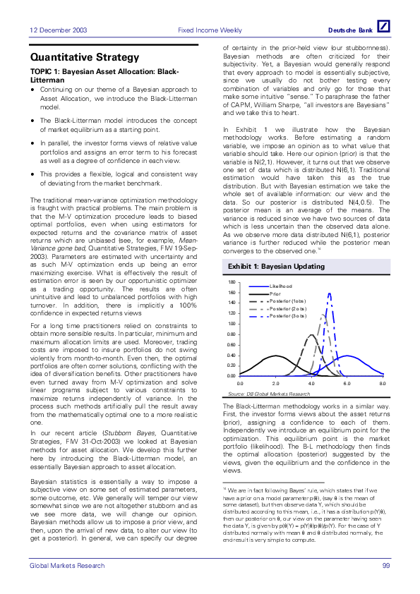In Exhibit 1 we illustrate how the Bayesian methodology works. Before estimating a random variable, we impose an opinion as to what value that variable should take. Here our opinion (prior) is that the variable is N(2,1). However, it turns out that we observe one set of data which is distributed N(6,1). Traditional estimation would have taken this as the true distribution. But with Bayesian estimation we take the whole set of available information: our view and the data. So our posterior is distributed N(4,0.5). The posterior mean is an average of the means. The variance is reduced since we have two sources of data which is less uncertain than the observed data alone. As we observe more data distributed N(6,1), posterior variance is further reduced while the posterior mean converges to the observed one.14 Exhibit 1: Bayesian Updating 1.80 Likeliho o d 1.60 P rio r 1.40 P o sterio r (1o bs) P o sterio r (2 o bs) 1.20 P o sterio r (3 o bs) 1.00 0.80 0.60 0.40 0.20 0.00 0.0 2.0 4.0 6.0 8.0 Source: DB Global Markets Research The Black-Litterman methodology works in a similar way. First, the investor forms views about the asset returns (prior), assigning a confidence to each of them. Independently we introduce an equilibrium point for the optimization. This equilibrium point is the market portfolio (likelihood). The B-L methodology then finds the optimal allocation (posterior) suggested by the views, given the equilibrium and the confidence in the views. 14 We are in fact following Bayes’ rule, which states that if we have a prior on a model parameter p(θ), (say θ is the mean of some dataset), but then observe data Y, which should be distributed according to this mean, i.e., it has a distribution p(Y|θ), then our posterior on θ, our view on the parameter having seen the data Y, is given by p(θ|Y) = p(Y|θ)p(θ)/p(Y). For the case of Y distributed normally with mean θ and θ distributed normally, the end-result is very simple to compute. 99 Deutsche Bank@ Fixed Income Weekly This leads to more stable, tractable and intuitive portfolios. In particular transaction costs are greatly reduced since the effects of our views is mitigated by the inclusion of the equilibrium. Exhibit 2: Black-Litterman Methodology Strategic Tactical • Global risk aversion • Markert capitalization weights • Covariance matrix (Σ) • Investor‘s active views • Confidence in views 12 December 2003 every single asset. On the other hand, with traditional M-V analysis, one can only express absolute views and has to do so for every single asset. As such we have one absolute view on the 10+Y bucket. In addition we have two relative views on the steepness of the short term and medium term parts of the curve. Table 2 summarises the views as relative value portfolios. Table 2: Investor Views Market implied returns Distribution of views (Prior distribution) Normal (Π, Σ) Normal (V, Ω) 1-3 Y 3-5 Y 5-7 Y 7-10 Y 10+ Y Views Equilibrium View 1 1.00 -1.00 0.00 0.00 0.00 -0.20% -0.34% View 2 0.00 0.00 1.00 -1.00 0.00 -0.25% -0.25% View 3 0.00 0.00 0.00 0.00 1.00 1.80% 1.91% Source: DB Global Markets Research Combining Views with the equilibrium Posterior Distribution The extent to which we deviate from the market equilibrium will depend on how far our views are from it and the degree of confidence we have in our views. Normal (combined Π and V, combined Σ and Ω) Source: DB Global Markets Research, K.Iordanis The market equilibrium To derive equilibrium returns, we make the assumption that the market is efficient. It has often been demonstrated that historically, the market portfolio was very different from the ex-post optimal one. However we pointed out in our recent articles that the market portfolio was not statistically different from the optimal one. On this assumption, the equilibrium returns π are15: π = δΣW where: δ is the global coefficient or risk aversion Σ is the covariance matrix of asset returns W are the market weights of the assets For example, looking at the market for Bunds, we derive the equilibrium returns given in table 1 (we assume that δ=7). The Black-Litterman returns are derived using the standard Bayesian updating formula with the investor views as the prior and the market equilibrium as the observed data16. Our views imply lower returns in general. Indeed, our only absolute view states that the 10+Y bucket will not perform as well as implied by the market. Because assets are positively correlated, this view will negatively affect returns of other assets. Indeed, even though view 2 is in line with the equilibrium, the other views imply lower returns for 5-7Y and 7-10Y buckets. Because view 1 is relative, it does not affect absolute return levels to the same extent. It implies that the 1-3Y bucket will outperform the 3-5Y bucket more than is implied by the market. For that reason the expected return of the 1-3Y bucket, decreases much less than that of the 3-5Y bucket. We see in Exhibit 3 that these effects are greater, the higher our confidence in our views. Table 1: Market Equilibrium Buckets Weight 1-3 Y 3-5 Y 5-7 Y 7-10 Y 10+ Y 27.94% 20.62% 14.01% 23.39% 14.04% Volatility 1.21% 2.60% 3.63% 4.65% 8.35% Excess Return 0.26% 0.60% 0.87% 1.13% 1.91% Source: DB Global Markets Research Investor’s Views One of the main advantages of the Black-Litterman approach is in the formulation of own views. Views can be relative or absolute (view on the return of only one asset). In addition we do not have to express a view for 15 If the market is efficient, the market maximises the following utility function with respect to the weights W: U(W) = W*π - ½δ W’ΣW This implies that U’(W) = 0 or π - δΣW = 0 ⇒ π = δΣW 100 16 Formally we have Bayes’ rule applied to our expected returns: pdf(E(r)/π) = pdf(π/E(r)) pdf(E(r)) / pdf(π) Global Markets Research 12 December 2003 Fixed Income Weekly Exhibit 3: Black-Litterman varying degree of confidence Returns with 1.60% 1.40% 1.20% transparency of construction. Necessarily, it means we will only be forming optimal portfolios in Euroland. Our views are not extreme and merely a summary of our strategy and RV calls on Euroland yield curves and asset classes. Essentially, we have the following views: 2.00% 1.80% Equilibrium • Lo w-Co nf M id-Co nf • Hi-Co nf • 1.00% • 0.80% 0.60% • 0.40% 0.20% 0.00% 1-3 Year 3-5 Year 5-7 Year 7-10 Year 10+ Year Source: DB Global Markets Research Consistent with these expected returns, we see that funds flow mainly to the 1-3Y bucket. Funds flow mainly out of the 3-5Y and 5-7Y buckets since their expected returns decrease a lot with our confidence (especially in relative terms). Exhibit 4 shows the full picture. Exhibit 4: Optimal Weights with varying degree of confidence 50% B enchmark 45% Lo w-Co nf 40% M id-Co nf 35% Hi-Co nf 30% 25% 20% 15% 10% 5% 0% 1-3 Year 3-5 Year 5-7 Year 7-10 Year 10+ Year Source: DB Global Markets Research The Black-Litterman model therefore provides a method to obtain expected returns that take into account the uncertainty in the investor’s view and the market equilibrium. It offers a greater degree of flexibility since we can express different degrees of confidence in the different views. As already mentioned one can express relative and absolute views on any combination of assets. Because it introduces the market equilibrium it provides investors with neutral implied expected returns on assets for which he does not have views. Optimal portfolios We concentrate on the set of assets for which we have an abundance of data. In particular, we will use the iBoxx indices for Euro-denominated bonds due to their ease of use, relatively long time-series, and Global Markets Research Deutsche Bank@ • • • • • • Neutral on duration, Long 2-10 steepeners Neutral on 10-30 steepeners Long 5Y vs 2Y and 10Y Long the condor: 2Y-30Y flatteners vs 5Y-10Y steepeners Wideners on Bund ASW Wideners on Bund-OAT spreads Wideners on Bund-BTP spreads Neutral on Bund-SPGB Spreads Wideners on Bund-Jumbo Pfandbriefe spreads Tighteners on Bund-Corporate spreads While this may seem an abundance of views, due to our relative confidence in each, we are able to balance them to output a portfolio. Each of our views on spreads will be combined with the carry of the given index or portfolio of indices to give us an expected return, which is in turn combined with the equilibrium expected return according to the BlackLitterman method. We then optimise with budget constraints, no-short constraints and a tracking-error target. We give a portfolio for a very modest tracking error of 10bp annually (reflecting our modest experience in the use of our model). As the year proceeds, we will increase our allocation, but the discerning should be able to scale our views to attain a more risky portfolio allocation. As can be seen, the results are not entirely surprising but should require some further clarification. The fact that Austria, Ireland, Portugal benefit from relatively low correlations to other asset classes, should make them preferred to some extent, for diversification benefit, yet these advantages can be counterbalanced by the relative attractiveness of other sectors. Netherlands and Finland each have much higher correlations (especially to the 1-3Y, 3-5Y, and 5-7Y buckets in Germany, France and Italy). The fact that they correlate better with the short-end effectively supports our steepening view (although it is not reflected in our maturity bucketing in Exhibit 4, which only reflects the maturity buckets of the core sovereigns and the jumbos). Spain is more highly correlated to the short-end of France and thus the underweight of Spain can be linked to the underweight in France. Finally, Italy is overweight 101 Deutsche Bank@ Fixed Income Weekly merely because of the attractive spread pickup, in spite of the relative widening of Bund-BTP spreads. Exhibit 3: Sector Under/Overweights Austria -0.434% Belgium 0.398% Finland 0.034% France -0.083% Germany 0.027% Ireland -0.022% Italy 2.215% Netherlands 1.277% Portugal -0.062% Spain -1.030% Sub Sov 0.033% Jumbo -3.348% Corporates 1.000% Source: DB Global Markets Research The correlation between Subsovereigns and Jumbos means that the underweight of Jumbos will generally have a small resulting underweight on Subsovereigns (unless we had had a conflicting view, of course). As we mentioned above, due to the fact that the standard iBoxx indices will only break down core Euroland sovereigns and Jumbos by maturity means that we have only reported them in Exhibit 4. Exhibit 4: Maturity Under/Overweights (Core Sovereigns and Jumbos) Bucket 1-3Y 3-5Y 5-7Y 7-10Y 10+Y Weights -2.862% 4.344% 0.642% -3.514% 0.201% 12 December 2003 directions include a more religious application of Bayes’ rule, where we juggle a tactical prior given by our RV views (combined with data to give a posterior) and our strategic prior given by our equilibirum model (combined with data to give a posterior), finally combining the two models via Bayesian Model Averaging. Appendix: The Black-Litterman formula The market implied expected Returns (ER) are uncertain since they are unobserved: ER = π + ν Where ν ~ MVN(0, τΣ). It represents the confidence in the equilibrium. τ is a (small) scaling factor such that 0 < τ < 1reflecting the fact that the variance in the expected returns is smaller than the variance of the actual returns. Our views are expressed as relative value portfolios to which we assign a return and a variance. P’(ER) = Q + ε Where ƒ P is an nxk matrix of linear restrictions. They give the combinations (portfolios) of assets for which we have a view. We have k≤n views. ƒ Q is a kx1 vector of our view of expected returns ƒ ε is a kx1 vector of errors. ε ~MVN(0, Ω) ƒ Ω is a diagonal kxk matrix of confidences in our views. Each entry represents the confidence in each of our views. A lower entry represents a higher confidence Source: DB Global Markets Research Focusing on the core and Jumbo weights by maturity, we see that the butterfly tends to have a larger influence. We note of course, as we mentioned above, that our overweights in Netherlands and Belgium will effectively change the relative maturity weighting of the entire portfolio towards a much more short position. This to a small extent can be seen in the duration of the optimal portfolio, which at 5.00 yrs vs 5.05 yrs for the index, indicates that, in spite of our neutral duration stance, our steepener tends to favour slightly shorter duration asset classes. We might mention that some of our outcomes may be a result of having too few views, and the fact that any one asset class can be favoured mostly from correlation effects rather than an explicit view may be a deficit of the approach and force us to take more explicit views on individual sovereign spreads. Conclusions We will seek to utilize the Black-Litterman framework over coming months in Europe. Since this is not the final chapter in asset allocation methods, we will we will also seek to improve upon the method. Indications are that by expressing uncertainty over the covariance, we can gain some more flexibility and make our assumptions somewhat more intuitive. Other possible 102 We therefore have the following system of equations: π = ER + ν Q = P’ER + ε π  Y =  , Q Setting: I X =  ,  P' u ~ MVN (0,V ), τΣ 0   V =   0 Ω We have: Y = X(ER) + u, so using GLS (Generalised Least Squares)17: -1 -1 -1 ER = (X’V X) X’V Y  ER = (I   ( τΣ 0   P )  0 Ω  ER =  (τΣ) −1  [ PΩ −1 )  I     P'   I     P '  −1 ] [(τΣ) ER = (τΣ) −1 + PΩ −1 P ' 17 −1 −1 −1 ((τΣ) −1 τΣ 0   P )  0 Ω (I −1 ) −1 π  PΩ −1   Q π + PΩ −1Q ] π    Q Satchell and Showcroft (1997) derive the full pdf of ER using bayes theorem: pdf(ER|π) = pdf(π|ER)pdf(ER)/pdf(π) Global Markets Research 12 December 2003 Deutsche Bank@ Fixed Income Weekly We comment that these updating formulas are the same as the standard Bayes’ rule where we have a prior on some elements of a regression beta, given by ER (our prior, P' ER ~ N (Q, Ω) ), and we observe normally distributed data (in this case ER ~ N (π , τΣ) ) and can determine the posterior mean (as reported above) and variance as needed by standard formulas. Exhibit 1: Equal weighted butterflies do not exhibit mean reversion Daniel Blamont (44) 20 7547 5106 Nick Firoozye (44) 20 7545 3081 TOPIC 2: Butterflies: just another way of taking a view on slopes? • We have already established that equally weighted butterflies, especially in Euroland, do not exhibit mean reversion, thus taking views on these butterflies is difficult. • In this article, we establish the link between forward slopes and butterflies, with moneymarket slopes linked to 2-5-10 and a whole host of related butterflies and long-end butterflies related to forward steepeners/flatteners. • Thus, taking views on the intricacies of curve shape is entirely taking views on the course of the central bank’s policy (for short-butterflies) and on the slope (for long-term butterflies). Also, butterflies and slopes sometimes do go out of line, and we present RV strategies for taking advantage of their relative mispricings. • We present a few views as elaboration of our USD EUR 2-4-7 -1.69 -2.48* 2-5-10 -1.72 -2.08 2-7-12 -1.15 -1.00 3-7-12 -1.30 -1.06 4-9-12 -0.97 -1.21 5-9-12 -1.09 -1.53 5-10-15 -1.39 -1.54 5-15-30 -0.71 -1.49 7-9-12 -6.49*** -4.50*** 7-10-15 -6.02*** -2.68* 10-15-30 -0.89 -2.16 10-20-30 -0.70 -1.77 Note *** Mean reverts at 1% confidence level ** Mean reverts at 5% confidence level * Mean reverts at 10% confidence level • We find that taking a view on 2-5-10 and 10-2030 butterfly is usually sufficient to take a view on the entire spectrum of butterflies. Butterfly We also showed that market-neutral butterflies showed some more hope of mean-reversion, especially in the US. In Europe, unfortunately, even these market-neutral butterflies proved non-mean-reverting, save for a few extremely closely spaced “flyettes” (e.g., 2-4-5, 3-4-5, or involve the specialness of the 7Y point). Nonetheless, even in the case of the US, we would probably be unwise to expect mean-reversion of most market-neutral butterflies to occur over all periods and histories. In fact, most research tends to indicate that there are three common trends18 or principal components which drive yields. We find, admittedly a bit surprisingly, a fundamental difference between the US and Euroland - the third principal component has been mean reverting in the US but not in Euroland – strategic overweight 5Y versus 2-10 in Euroland. 18 In our last Quantitative Strategy (FIW 21-Nov-03), we established that almost all equal weighted butterflies, both in the US and Europe failed to be mean-reverting in any meaningful way. In other words, while we could establish half-lives, the uncertainty indicated that within a 95% or 99% confidence interval, the half-life could have been infinite. The table below shows the results of the Dickey-Fuller test on some of the commonly traded butterflies, where only large test-statistics indicate that mean-reversion parameters are significant. A stochastic common trends model (a la Stock-Watson) indicates that yields are linear combinations of a set of unit-root (random walk) factors plus a (stationary) error term ε, which are either iid or mean-reverting: y = LFt + ε t Ft = Ft −1 + δ t where δ is assumed to be independent of ε, and this is typically estimated by Kalman-Filters. Estimating a stochastic common trends is is essentially like doing PCA in levels (i.e., ) Ft ≈ ( L' L) −1 L' yt ). In almost all studies the yield curve is thought to be driven by three trends: level slope and curvature, or the first, second and third modes of yields, and that only fourth and higher modes are truly mean-reverting. Stochastic common trends models are just another form of a cointegration or vector-errorcorrection model (Engle-Granger, Johannsen) ∆yt = αβ ' yt −1 + ε t (with a different ε) where attention is now on the mean-reverting component β’yt-1, which is orthogonal to the common trends (i.e., β ' yt ⊥Ft ), or in other words, the cointegration relations are just the higher modes and are mean-reverting. The condor trade (see When good condors turn bad, Quantitative Strategy, FIW 8-Nov02, and this week’s EUR Government Bonds section) is an example of a trade which depends only on the cointegration relation, i.e., it is subject only to the fourth principle component and thus is known to be mean-reverting. Global Markets Research 103 Deutsche Bank@ Fixed Income Weekly thus explaining the relatively well behaved nature of butterflies in the US. 12 December 2003 Fed funds rate (lhs inverted) 0 2-10 slope Jan-94 Butterflies: just another call on slopes? Source: DB Global Markets Research While there has been much said about the relationship of equally-weighted butterflies, the 2-5-10 in particular, with the slope of the money market curve, the reasons for the connection are still somewhat nebulous. Exhibit 2: 2-5-10 butterfly – is it just money market slope? MM slope 3Mx1Y - 3Mx3M (lhs) 120 250 2 200 3 150 4 100 5 50 6 0 7 -50 Dec-95 Nov-97 Nov-99 Oct-01 The butterfly, on the other hand, mostly takes the absolute level of rates out of the picture. We can see that as well from Exhibit 3, where butterfly spreads seem to exhibit no exact correspondence to absolute levels. A similar relationship holds for Euroland. Exhibit 4: 2-5-10 butterfly and the level of rates –not as strong a relationship Fed funds rate (lhs inverted) 0 15 2-5-10 butterfly 10 40 2 60 5 40 30 3 0 20 20 4 10 -5 0 5 0 -10 -20 6 Aug-00 Mar-01 Oct-01 May-02 Dec-02 Jul-03 Source: DB Global Markets Research Essentially, we can think of the five year as a leveraged bet on the direction of rates. While 2Y-10Y slopes are steeper when the output gap is higher (or generally when absolute level of short-rates are low—a striking correspondence in the case of the US, see Exhibit 3), the slope tells little about the market’s implied expectations over the direction of short rates. Yes, steep slopes, typically coincident with poor economic conditions, tend to flatten in time and short rates come back to normal levels (see Treasury Slope and Economics, FIW, Quantitative Strategies, 23-Aug-02, for a link between slope and economic fundamentals, e.g., the output gap). Yet, slope is exceptionally persistent and steep slopes tend to be followed by steep slopes (another manifestation of the forward bias). Indeed, steep slopes indicate that rates are expected to rise, somewhat, but also that term premia are high in general. Exhibit 3: US 2-10 slope, just another view on levels? 104 -10 -15 -40 Jan-00 60 50 1 80 Sep-03 20 2-5-10 butterfly 100 300 1 But all is not lost, as showed in the previous publication, a view on just a few simple butterflies (e.g., 2-5-10, and 10-15-20), either equally weighted or market-neutral, is sufficient to take a view on every other commonly traded butterfly. The problem of how to establish views on these few butterflies is easily overcome as we show below that most butterflies are in fact, calls on slopes or money-markets. To the extent that one disagrees with the risk-neutral or market perception of the direction of rates, one would necessarily have a corresponding view on a wide range of butterflies. 350 7 Jan-94 -20 Dec-95 Nov-97 Nov-99 Oct-01 Sep-03 Source: DB Global Markets Research Rather than revealing the absolute level of rates or the market’s take on the economic outlook, the butterfly tells more about the market’s implied view on the direction of short-term interest rates. The five year is, in some ways, a proxy for the entire market, since the duration of both US and EUR bond markets are each close to that of the 5Y bonds. If this is entirely the rationale, of course, we should see the specialness of the 5Y point being shifted to shorter maturities as the US retires its 30Y or as the MBS market duration contracted during the not-so-distant days of rallying bond markets. This is not easy to either verify or reject. Nonetheless, the 5Y seems a focal point and buyers of the market tend to focus on the 5Y before they shift attention to the entirety of the rest of the market. The same goes for sellers. Thus the relative richness/cheapness of the 5y sector should reflect markets expectation of the future movement of rates. The link between butterflies and market expectations is evident when comparing to the short end of the curve, where the butterfly premium shows a very large Global Markets Research Deutsche Bank@ Fixed Income Weekly correlation to the slope of the money market curve. And, while steep money-market curves do indicate the presence of a term-premium, (see Euroland Strategies, FIW 16-May-2003, for a discussion of the termpremium in money-markets), the effect is much more muted than in longer-slopes and money-markets can be used to a large degree to discern the market’s view on the direction of rates. Our interest then is to establish which slopes are most closely related to some of the more-frequently traded butterflies. And, the results should be two-fold: a) Establish view or measure risks on butterflies through our views on the outlook of rates b) to establish dislocations in the relationship between butterflies and slope and look for trading opportunities. In Europe in particular, we believe the money-market curve is far too cheap at the long end and our view is that the ECB will have to remain on hold (with risks of a cut due to an appreciating Euro). We can monetise this view through our 2-5-10 butterfly position. This is especially relevant for real money accounts who can express a long money market view through a 2-5-10 butterfly. Exhibit 5 shows the correlation between money-market slopes and some commonly traded butterflies. Although the 3Mx3M versus the 1Yx3M has been the source of some focus in its relation to the 2-5-10, at 88% correlation in US and 84% in EUR, it is far from the most attractive combination (all figures quoted below are from 2000 onwards). Exhibit 5: Short butterflies relate to slopes of forwards* forward slopes (e.g., 3M forwards of 2Y-10Y, etc) to longer butterflies and find the correspondence is high Exhibit 6: Long butterflies relate to forward slopes 5-10 slope 10-30 spot slope spot 3M fwd 3M fwd 5-10-15 0.99 0.93 0.98 0.91 5-10-20 0.89 0.76 0.87 0.94 10-20-30 0.98 0.99 0.99 0.99 12-20-30 0.97 0.99 0.98 0.98 5-10-15 0.94 0.60 0.91 0.59 5-12-15 1.00 0.79 0.99 0.78 10-20-30 0.90 0.94 0.93 0.95 12-20-30 0.84 0.91 0.88 0.95 US Source: DB Global Markets Research In fact, we see the 10-20-30 butterfly shows a very strong relationship with the 10Y-30Y slope 3M forward (see Exhibit 7). Exhibit 7: Correlation between the EUR 10-2030 butterfly and the forward slope 50 y = 0.3574x + 3.5282 R2 = 0.9022 40 30 20 10 0 -10 -50 US 6M-2Y 3M-1Y 3M-2Y 1Y-2Y 3-5-7 0.95 0.74 0.93 0.96 2-5-10 0.91 0.88 0.93 0.84 2-4-7 0.78 0.88 0.82 0.65 4-7-10 0.91 0.86 0.81 0.96 EUR 3-5-7 0.87 0.67 0.89 0.76 2-5-10 0.71 0.84 0.87 0.25 2-4-7 0.56 0.84 0.72 0.70 4-7-10 0.85 0.74 0.81 0.89 *The underlying for the above table is the 3M rate Source: DB Global Markets Research But, if 2-5-10 is linked to this short-end slope of money markets, we should expect that something like 4-7-12 should be related to a slightly longer slope, for example, a 2Yx3M vs a 3Yx3M. This is to some extent the case, but, as we mentioned earlier, looking at long forwards with a 3M underlying will, probably be more an indicator of the level of term premium than just the market’s view of the direction of short rates. What about the butterflies at the long end? Interestingly, we find that a view on long end butterflies is again a view on the slope. In Exhibit 6, we relate the Global Markets Research 5-10 slope 10-30 slope EUR 10-30 slope 3m fwd 12 December 2003 0 50 100 150 10-20-30 butterfly Source: DB Global Markets Research The above chart speaks for itself – a view on the 10-2030 butterfly is, essentially, a view on the forward 10-30 slope. As we had shown in the Quantitative Strategies of FIW 21-Nov-03, other commonly traded butterflies are found to be cointegrated either with the 2-5-10 or the 10-20-30 butterfly. Thus having a view on the 2-5-10 or the 10-20-30 butterfly is normally sufficient to have a view on the entire butterfly spectrum. As a risk-taker, this should be enough. One should generally have views on the directions of rates relative to forwards or perhaps on the directions of slopes relative to given forwards. It also enables any professional risk-manager the ability to dissect a trade into a set of calls on spot slope and levels. For instance, 10-20-30, a call on 3Mx10Y vs 3Mx30Y, can be thought of as a call on 10Y-30Y slope and on short-rates. A bearish duration call combined (since 10-30 slope flattens when the 10Y sells off in Europe) combined with an ECB on hold should necessarily mean 20Y richening relative to the wings. 105 Deutsche Bank@ Fixed Income Weekly Trading the dislocation: can we monetise it? Next, we explore the relative value opportunities between butterfly and slope trades. The table below shows the half life of dislocations between butterfly and slopes. The low half lives makes these attractive contenders for relative value trades. The fact that, in spite of the high R-squares, dislocations can actually be large enough to monetise, leads us to believe that this is a valid set of relative value trading strategies. Exhibit 8: Half lives of dislocations between butterflies and slope Butterfly Slope Half life of residuals (days) US EUR 2-5-10 3mx1Y – 3mx3m 15 10 2-4-7 3mx1Y – 3mx3m 15 7 10-20-30 30Y – 10Y spot 5 21 5-10-15 3Mx10Y – 3Mx5Y 8 22 12 December 2003 A view on equally weighted butterflies is essentially a view on the slope. We find that the short to medium tenor butterflies exhibit strong correlations with the slope of the money market curve. Thus a view on the 25-10 butterfly is essentially a view on the slope of the money market curve. The long end butterflies tend to be correlated with the 10-30 slope, either spot or forward, thus enabling a trading view for these butterflies. Nick Firoozye (44) 20 7545-3081 Mohit Kumar (44) 20 7545-4387 Source: DB Global Markets Research In Exhibit 9, we see that residuals from our level regressions, as in the 2-5-10 vs the money-market curve, that the dislocations have a standard deviation of 3bp. Assuming a 1bp bid-offer on 2-5-10, and a 0.5bp bid-offer on each Euribor future, we should still be provided with sufficient opportunities for trades even if this indicator does not lead us to take positions every day. Exhibit 9: In spite of high R-squares, mispricings can still be advantageous 10 8 resdiuals (bp) 6 4 2 0 -2 -4 -6 -8 Jan-00 Dec-00 Dec-01 Nov-02 Nov-03 Source: DB Global Markets Research So what can we conclude? In our two articles on butterfly trades, we have outlined a methodology for taking view on butterfly trades. We showed in the last article, that for market neutral butterflies, we need to take into account the half life, its standard error (i.e., whether or not it is mean-reverting), and the standard deviation of the residuals in order to evaluate the attractiveness of a butterfly19. 19 We showed that the attractiveness of a butterfly can be measured by looking at the ex-ante Sharpe ratio defined as E[ Dislocation] + carry Sharpe ratio = σ 106 Where E[Dislocation] is the expected mean reversion in the butterfly residuals, carry is the butterfly carry over the investment horizon and σ is the standard deviation of the butterfly residuals. Global Markets Research