547
Brazilian Journal of Physics, vol. 39, no. 3, September, 2009
A 3-D four-wing attractor and its analysis
Zenghui Wang∗
F’SATIE, Department of Electrical Engineering, Tshwane University of Technology, Pretoria 0001, South Africa and
Department of Automation, Shandong University of Science & Technology, Qingdao 266510, China
Yanxia Sun,† Barend Jacobus van Wyk, and Guoyuan Qi
F’SATIE, Department of Electrical Engineering, Tshwane University of Technology, Pretoria 0001, South Africa
Michael Antonie van Wyk
School of Electrical and Information Engineering, University of the Witwatersrand, Johannesburg 2000, South Africa
(Received on 14 April, 2009)
In this paper, several three dimensional (3-D) four-wing smooth quadratic autonomous chaotic systems are
analyzed. It is shown that these systems have a number of similar features. A new 3-D continuous autonomous
system is proposed based on these features. The new system can generate a four-wing chaotic attractor with less
terms in the system equations. Several basic properties of the new system is analyzed by means of Lyapunov
exponents, bifurcation diagrams and Poincare maps. Phase diagrams show that the equilibria are related to the
existence of multiple wings.
Keywords: Chaos; four-wing attractor; Lyapunov exponents; bifurcation.
1.
INTRODUCTION
Since Lorenz discovered a simple three-dimensional
smooth autonomous chaotic system in 1963 [1], it was found
that chaos is very useful in many application fields such
as engineering, medicine, secure communications, and so
on. Much research was done in this field [2, 3]. Creating
a chaotic system with a more complicated topological
structure such as a multi-scroll or multi-wing attractor,
therefore, becomes a desirable task and sometimes a key
issue for many engineering applications. In this endeavor,
there are two major thrusts: generalizing Chua’s circuits
with multi-scroll attractors and generalizing the Lorenz
system with multi-wing attractors. In efforts to generalize
Chua’s circuit [4] to produce multi-scroll attractors, several
effective techniques have been developed, including generalized Chua’s circuits and cellular neural networks [5, 6].
In [4, 5, 7], the piecewise-linear (PWL) function method
was utilized, which can increase the number of equilibria
by adding breakpoints. A sine-function approach was then
proposed for creating multi-scroll chaotic attractors [8].
Later, a stair function was used for generating 3D-grid-scroll
attractors [9, 10]. More recently, several different nonlinear
functions including switching, hysteresis and saturated
functions were utilized for creating chaotic attractors with
multi-merged basins of attraction, or with multi-scroll
attractors [11–14]. Note that the aforementioned methods
for generating multi-scroll attractors have some common
characteristics [15, 16]:
(i) The nonlinearities of these systems are usually not
smooth functions; they are either piecewise-linear continuous functions or discontinuous ones such as the staircase
function, switching function, and hysteresis-series function.
(ii) The basic techniques either increase the number of
equilibria via PWL functions with more breakpoints, or use
∗ Electronic
† Electronic
address: wangzengh@gmail.com
address: sunyanxia@gmail.com
stair or hysterisis functions to realize equilibrium jumping.
(iii) The number of scrolls equals the number of equilibria.
(iv) The basic shape of the attractors is cyclic, called a scroll.
Another major thrust has been the generalization of the
Lorenz system [17]. Recently some new chaotic systems
were proposed, including the Chen system, the generalized
Lorenz system family, and the hyperbolic-type of generalized Lorenz canonical form [18–20]. Some four-dimensional
chaotic systems were also presented, which have more complicated dynamic properties than three-dimensional chaotic
systems, such as the system proposed in [21]. It can be seen
that the characteristics of generalized Chua’s circuits are different from the generalized Lorenz systems. For example,
the nonlinearities of these systems are usually smooth functions, the number of wings is not equal to the number of
equilibria and the basic shape of the attractors is a butterfly,
called a wing [15, 22]. Qi proposed two four-wing chaotic
attractors produced by 4-D systems with complicated structure [16, 22].
In fact, most of the multi-scroll attractors were generated
by increasing the breakpoints in the non-linearity. Recently,
a four-wing or three-wing butterfly attractor was generated
from a three-dimensional system [23] by relying on two embedded state-controlled binary switches. However, these systems are usually not smooth systems.
It would be very exciting to construct a lower-dimensional
chaotic system which has less terms in the system equations, but with a complex attractor structure. To generate
multi-wing chaotic attractors from a three-dimensional (3D) smooth system remains a technical challenge, especially
if a simple structure is a pre-requisite. In this paper, we
analyze several proposed smooth quadratic autonomous 4wing chaos systems and present a new 4-wing chaotic system whose number of linear and quadratic terms is less than
existing 4-wing chaotic systems. In the following sections,
the new system is investigated by means of the Lyapunov exponent spectrum, Poincare maps and bifurcation diagrams.
�548
Zenghui Wang et al.
(a) Projection on the x − y plane
(c) Projection on the y − z plane
(b) Projection on the x − z plane
(d) 3-D view by ’.’ in the x − y − z space
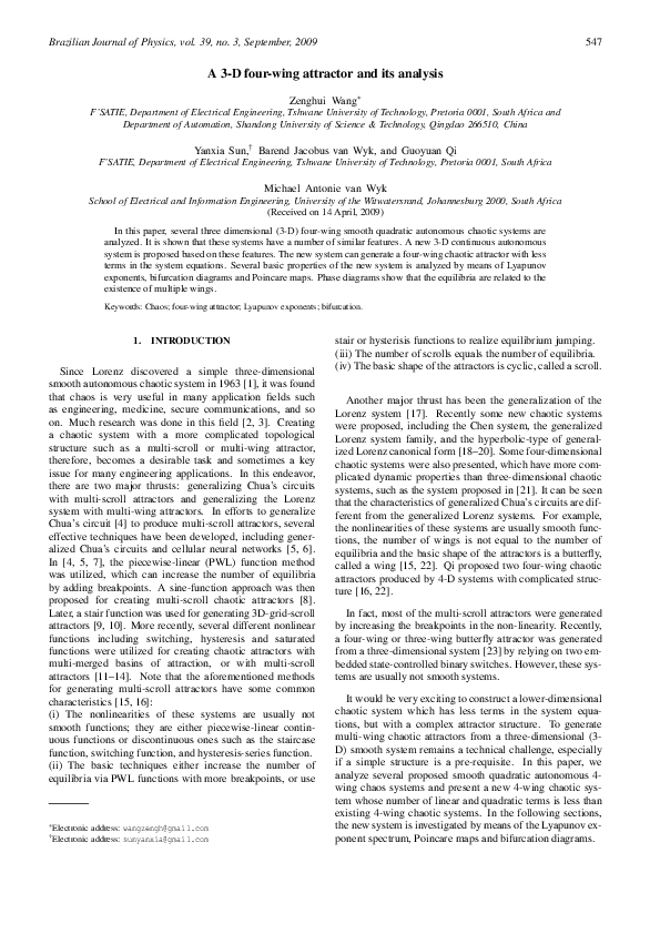
FIG. 1: Four-wing chaotic attractor, with a = 0.2, b = −0.01, c = 1, d = −0.4, e = −1.0 and f = −1.
2.
3-D FOUR-WING SMOOTH AUTONOMOUS CHAOTIC
SYSTEMS
and closely located double-wing attractors [26]. In [27], a
3-D autonomous quadratic system was reported, which can
generate a single four-scroll attractor. For the simplicity of
comparison, the system is parameterized as
ẋ1 = a1 x1 − y1 z1 + a2 ,
ẏ1 = b1 y1 + x1 z1 ,
ż1 = c1 z1 + x1 y1 ,
(1)
where a1 , a2 , b1 , c1 are real constants. If
⎧
b c > 0,
⎪
⎪
⎨ 1 1
�= 0,
a1 √
a
b1 c1 < min(−a2 , a2 ) if b1 > 0,
⎪
1
⎪
⎩ √
a1 b1 c1 > max(−a2 , a2 ) if b1 < 0,
there are five equilibria in this system, given by
FIG. 2: The bifurcation diagram of the system (6) with respect to b,
and with a = 0.2, c = 1, d = −0.4, e = −1.0 and f = −1.
In [24, 25], a three-dimensional smooth quadratic autonomous system which seemingly can produce a four-wing
attractor was proposed. At first, it was believed that this
system could produce a four-wing chaotic attractor, termed
a four-scroll attractor but this was then later shown by the
same authors to be a numerical artifact. It was not a real
four-wing chaotic attractor but consisted of two coexisting
a2
, 0, 0),
a1
�
�
(−a2 − a1 p)b1
(−a2 − a1 p)b1
= (p, ±
p, ±
),
p
p
�
�
(a2 − a1 p)b1
(a2 − a1 p)b1
p, ±
),
= (−p, ∓
p
p
S0 = (−
S1,2
S3,4
√
where p = b1 c1 . As can be seen from the equilibria, there
is no trivial equilibrium caused by the constant input of first
�Brazilian Journal of Physics, vol. 39, no. 3, September, 2009
549
equation in (1). Consider the following transformation of
variables:
which can evolve into periodic and chaotic orbits in case of
different parameters. When proper parameters are chosen, a
single four-wing attractor and a single three-wing attractor
appears.
As can be seen from systems (2), (3), (4) and (5), there are
a number of similar features common to these chaotic systems:
(1)There is at least one quadratic term in every equation,
which means there is at least three quadratic terms in one
system.
(2)There are five equilibria when these chaotic systems display four wings.
(3)There are at least four linear terms, and there is at least
one linear term in every equation of these systems.
The logical question is whether there is any system exhibiting similar behavior, but with less linear and quadratic
terms than these systems.
x1 = x2 −
a2
.
a1
The system (1) can be reformulated as
ẋ2 = a1 x2 − y1 z1 ,
a2
ẏ1 = b1 y1 − z1 + x2 z1 ,
a1
a2
ż1 = cz1 − y1 + x2 y1 ,
a1
(2)
which has a trivial equilibrium and is equivalent to system
(1). Another example is given by
3.
A NEW 3-D FOUR-WING SMOOTH AUTONOMOUS
CHAOTIC SYSTEMS
Based on the above features, a new simpler chaotic system
ẋ = ax + cyz,
ẏ = bx + dy − xz,
ż = ez + f xy,
FIG. 3: The maximum Lyapunov exponent spectrum of the system
(6) with respect to b, and with a = 0.2, c = 1, d = −0.4, e = −1.0
and f = −1.
ẋ1 = a1 x1 + a2 y1 + y1 z1 ,
ẏ1 = b2 y1 − x1 z1 + b23 y1 z1 ,
ż1 = c3 z1 − x1 y1 .
(3)
(4)
called the Qi 3-D four-wing system, which can generate two
coexisting single-wing chaotic attractors and a pair of diagonal double-wing chaotic attractors. The system can also
generate a four-wing chaotic attractor with very complicated
topological structures over a large range of parameters.
Recently, Chen [29] presented a new three-dimensional
smooth quadratic autonomous chaotic system,
ẋ1 = a1 x1 + ky1 − y1 z1 ,
ẏ1 = −b1 y1 − z1 + x1 z1 ,
ż1 = −x1 − c1 z1 + x1 y1 .
is proposed. Here a, b, d, e ∈ R, c > 0 and f < 0 are all constants, c f �= 0, and x, y, z are the state variables. If the system
is dissipative, ∇V = ∂xẋ + ∂yẏ + ∂żz = a + d + e should be less
than zero, that is, a + d + e < 0. This implies that a volume
element V0 is contracted by the flow into a volume element
V0 e(a+d+e)t in time t.
Theorem 1 If b = 0, the system (6) can not generate a fourwing chaotic attractor.
When a1 = 0.5, a2 = 0.15; b2 = −12.2, b23 = 1.0, c3 =
−8.79, the system has a real four-scroll attractor with eight
cross product terms on the right [28].
Qi [15] introduced a 3-D quadratic autonomous system
ẋ1 = a1 (y1 − x1 ) + e1 y1 z1 ,
ẏ1 = c1 x1 + d1 y1 − x1 z1 ,
ż1 = −b1 z1 + x1 y1 ,
(6)
Proof : This theorem can be proved according to different
cases in parameter space.
Case 1: c < 0
If b = 0, consider the first and the second equations of (6),
i.e.
ẋ = ax + cyz,
ẏ = dy − xy.
(7)
(8)
By multiplying both sides of (7) by x and of (8) by cy, respectively, the two equations become
ẋx = ax2 + cxyz,
cẏy = cdy2 − cxyz.
(9)
(10)
By adding both sides of (9) and (10), one obtains
ẋx + cẏy = ax2 + cdy2 .
(11)
Equation (11) is equivalent to
(5)
d(x2 + cy2 )
= 2d(x2 + cy2 ) + (2a − 2d)x2 .
dt
(12)
�550
Zenghui Wang et al.
Solving the above equation yields
�
�Z t
2
2
2dt
−2dt
2
2
2
x + cy = e
e
(2a − 2d)x dτ + (x0 + cy0 ) ,
0
(13)
where x0 and y0 are√
the initial state of system (6).
If a > d and |x0 | > −c|y0 |, according to (13), one obtains
√
(14)
x2 + cy2 > 0 ⇒ |x| > −c|y|.
√
If |x0 | > −c|y0 | and z0 �= 0, then for any time t > 0, the
system trajectory in the x − y plane will never travel from
one domain x > 0 to another, x < 0, or vice versa. That is, if
x0 > 0, then there will always be x(t) > 0 for t > 0; if x0 < 0,
then there will always
√ be x(t) < 0 for t > 0. The same is for
a < d and |x0 | < −c|y0 |.
If the system can generate a four-wing attractor, then the
attractor will not depend on the initial state, that is , the
√ initial
state value√can be chosen arbitrarily, such as |x0 | > −c|y0 |
or |x0 | < −c|y0 |. It conflicts with the above analysis, so
it is impossible to be a four-wing attractor when c < 0 and
b = 0.
Case 2: c > 0
If f > 0, the same result can be got according to the first and
third equations of system (6).
If f < 0, the same result can also be got according to the
second and third equations of system (6).
The proof is thus completed.
3.1. Equlibria
The equilibria of system (6) can be easily derived by solving the three equations ẋ = 0, ẏ = 0, and ż = 0. There is one
trivial equilibrium.
Let
√
�
ae 1 bc + sign(a) b2 c2 − 4acd 2
,z =
, ze
ye =
cf e
2c
√
bc − sign(a) b2 c2 − 4acd
=
,
(15)
2c
where sign() is a sign function. If caef > 0, b2 c2 − 4acd > 0
and c �= 0, there are four nontrivial equilibria:
c
c
S1,2 = (∓ ye z1e , ±ye , z1e ), S3,4 = (∓ ye z2e , ±ye , z2e )
a
a
(16)
In this case, system (6) has five equilibria (including the
zero equilibrium). It means system (6) is not topologically
equivalent to the generalized Lorenz canonical form (GLCF)
[20] which have three-equilibria at most.
Remark 1 If caef < 0, b2 c2 − 4acd < 0 , there is no nontrivial
equilibrium for system (6).
3.2. Simple property of the trivial equilibrium
By linearizing system (6) at the origin (trivial equilibrium), one obtains the Jacobian
⎛
⎞
a 0 0
J0 = ⎝ b d 0 ⎠ .
0 0 e
The eigenvalues of matrix J0 are
λ01 = a, λ02 = d, λ03 = e.
3.3. Symmetry and similarity
It is obvious that the new system is symmetric about
z-axis,which can be easily proven via the transformation
(x, y, z) → (−x, −y, z). Equilibria S1 , S2 are also symmetric
with respect to the z-axis and the same goes for S3 , S4 .
The dynamics near the neighborhood of S1 , S2 is similar
to each other in system (6), this feature also applies to S3 , S4 ,
and is caused by the similarity of the Jacobians of S1 and S2
(S3 and S4 ).
To prove this, let Ji denote the Jacobian of Si , i = 1, · · · , 4,
namely
⎞
⎞
⎛
−cye
a
cz1e
c1 ye
a
cz1e
c
1 ⎠ , J = ⎝ b − z1
d
− ac ye z1e ⎠ ,
d
J1 = ⎝ b − z1e
2
e
a ye ze
c
c
1
1
e
e
f ye − f a ye ze
− f ye f a ye ze
a
cz2e
d
J3 = ⎝ b − z2e
f ye − f ac ye z2e
⎞
⎞
⎛
cye
−cye
a
cz2e
c
2 ⎠ , J = ⎝ b − z2
d
− ac ye z2e ⎠ .
4
e
a ye ze
c
− f ye f a ye z2e
e
e
where T = diag(−1
There is a transformation matrix T , so that
T
−1
J1 T = J2 , T
−1
J3 T = J4 ,
(21)
(18)
Remark 2 As a, d, e ∈ R, there is no imaginary eigenvalue
in (17), and a Hopf bifurcation does not exist near the trivial
equilibrium which is different to systems (2), (4) and (5). The
dynamics near the origin is simpler than for systems (2), (4)
and (5).
⎛
⎛
(17)
−1
(19)
(20)
1), and T is an orthogonal ma-
�551
Brazilian Journal of Physics, vol. 39, no. 3, September, 2009
(a) Projection on the x − y plane with an initial state
(1, 1, 1)
(b) Projection on the x − y plane with an initial state
(−1, −1, 1)
FIG. 4: Double-wing chaotic attractor of (6), with a = 0.2, b = 0, c = 1, d = −0.4, e = −1.0 and f = −1.
trix, since
T −1 = T T = T.
(22)
Let Vi = [vi1 , vi2 , vi3 ] be the matrix consisted of eigenvectors of Si , i = 1, · · · , 4, the following equations can be obtained:
T −1V1 T = V2 ,
T −1V3 T = V4 .
(23)
Remark 3 S1,2 and S3,4 are two distinct equilibrium-pairs,
and every equilibrium-pair has the same local stable, unstable and center manifolds.
4.
THE FOUR-WING CHAOTIC ATTRACTOR
4.1. Bifurcation analysis with respect to parameter b
When a = 0.2, b = −0.01, c = 1, d = −0.4, e = −1.0 and
f = −1, there are five equilibria in system (6), namely
S0
S2
S3
S4
=
=
=
=
(0, 0, 0), S1 = (−0.6214, 0.4472, 0.2779),
(0.6214, −0.4472, 0.2779),
(0.6437, 0.4472, −0.2879),
(0.6214, −0.4472, −0.2879).
As ∇V = ∂xẋ + ∂yẏ + ∂żz = a + d + e = −1.2 < 0, the system
is dissipative. In order to investigate the stability of all the
equilibria, we consider the Jacobian matrix with respect to
each equilibrium and calculate their eigenvalues. The results
are shown in Table I. Based on the eigenvalues, we know
that S0 , S1 , S2 , S3 and S4 are all saddle-focus nodes implying
that all the five equilibria are unstable.
In order to determine whether the system is chaotic or
not, Lyapunov exponents should be calculated. In this paper,
we use the efficient QR based method [30] to compute the
Lyapunov exponents or Lyapunov exponent spectrum. With
these parameter values, the corresponding Lyapunov exponents are λ1 = 0.064, λ2 = 0 and λ3 = −1.262 for system
(6) and the system exhibits the four-wing chaotic dynamics
which is shown in Fig. 1. The projections of the phase portrait on the x − y, x − z and y − z planes are shown in Fig.
1(a)-1(c), respectively. The 3-D chaotic attractor is shown in
Fig. 1(d).
The system equilibria Si , i = 1, · · · , 4, which are denoted
as red ‘*’, are located at the centers of the four wings of the
attractor, and the origin is indicated by the red symbol ‘o’,
which is in the center of the whole chaotic attractor shown
in Fig.1. It can be seen that there exist many orbits not only
around S1,2 , but also around S3,4 , and even around S1,3 and
S2,4 , which play an important role in forming the real fourwing attractor, since they effectively connect the four subattractors, which surround the four equilibria.
Fig. 3 shows the maximum Lyapunov exponent spectrum,
which corresponds directly to the bifurcation diagram shown
in Fig. 2. Seen from Theorem 1, the parameter b is a very
important factor to create a four-wing attractor. Fig. 2 shows
the bifurcation diagram of the state variable x, in which the
orbit starts from (1, 1, 1).
As can be seen from Fig. 2 and Fig. 3, the chaotic attractors are symmetrical about parameter b and the middle
point is b = 0, which implies that parameter b has little effect on the chaotic dynamics, except for causing system (6)
to exhibit a four-wing attractor.
There are two kinds of orbital dynamical attractors in systems (6), a local one and a global one. The local attractor
relies on the initial region of the orbit, which includes a sink,
some simple periodic orbits and a single-wing chaotic attractor. The global attractor, which includes some complicated
orbits around all equilibria, a double-wing chaotic attractor
and a four-wing chaotic attractor, does not rely on the initial
region of the orbit. An obvious illustration is the phase figures when b = 0. When a = 0.2, b = 0, c = 1, d = −0.4, e =
−1.0 and f = −1, the phase diagrams of (6) are shown in
Fig. 4. In Fig. 4(a), the initial state is (1, 1, 1) which is different from Fig. 4(b) with an initial state (−1, −1, 1). As can
be seen from Fig. 4, they can not generate four-wing chaotic
attractors when b = 0, satisfying Theorem 1, but create two
coexisting double-wing chaotic attractors.
�552
Zenghui Wang et al.
TABLE I: Eigenvalues of Jacobian matrixes for all equilibria.
S0
S1
λ1 = −0.4 λ1 = −1.36
λ2 = 0.2
λ3 = −1
λ2,3 = 0.08 ± 0.47i
S2
λ1 = −1.36
S3
S4
λ1 = −1.38
λ1 = −1.38
λ2,3 = 0.08 ± 0.47i λ2,3 = 0.09 ± 0.48i λ2,3 = 0.09 ± 0.48i
(a) Poincaré map on the crossing section x = −0.62
(c) Poincaré map on the crossing section z = 0.28
(b) Poincaré map on the crossing section y = −0.45
(d) Poincaré map on the crossing section z = 0
FIG. 5: Four-wing chaotic attractor Poincaré mappings: with a = 0.2, b = −0.01, c = 1, d = −0.4, e = −1.0 and f = −1.
4.2. Poincare map of the four-wing chaotic attractor
As an important analysis technique, the Poincaré map can
reflect bifurcation and folding properties of chaos. When a =
0.2, b = −0.01, c = 1, d = −0.4, e = −1.0 and f = −1, one
may take x = −0.62, y = −0.45, z = 0.28 and z = 0 as crossing planes, respectively, where x = −0.62, y = −0.45, z =
0.28 is near the elements of the equilibrium of system (6).
Fig. 5 shows the Poincaré mapping on several sections, with
several sheets of the attractors visualized. It is clear that
some sheets are folded and and indicates that the system has
extremely rich dynamics.
5.
CONCLUSION
Several 3-D four-wing smooth quadratic autonomous
chaotic systems were analyzed and it was found that these
systems have similar features related to the creation of four-
wing chaotic attractors. A 3-D continuous autonomous system with less terms was consequently introduced. Some
basic properties of the new system were also analyzed by
means of Lyapunov exponents, bifurcation diagrams and
Poincare maps. Phase diagrams showed that the equilibria
are related to the existence of several wings. The new system
is very convenient for understanding the dynamical behavior
of multi-wing chaotic systems.
6.
ACKNOWLEDGMENT
This work was supported by the grants: National Research
Foundation of South Africa (No. IFR2008111000017);
Tshwane University Research foundation, South Africa;
the Natural Science Foundation of China (No. 10772135,
60774088); the Scientific Foundation of Tianjin City, China
(No. 07JCYBJC05800) and the Scientific and Technological
Research Foundation of Ministry of Education, China (No.
�Brazilian Journal of Physics, vol. 39, no. 3, September, 2009
553
207005).
[1] E. N. Lorenz, J. Atmos. Sci. 20, 130 (1963).
[2] A. S. de Paula and M. A. Savi, Brazilian Journal of Physics
38, 536 (2008).
[3] D. M. Maranhao and C. P. C. Prado, Brazilian Journal of
Physics 35, 162 (2005).
[4] L. O. Chua, M. Komuro and T. Matsumoto, IEEE Trans Circuits Syst-I 33, 1072 (1986).
[5] L. O. Chua and T. Roska, IEEE Trans Circuits Syst-I 40, 147
(1993).
[6] J. A. K. Suykens and L. O. Chua, Int. J. Bif. Chaos 7, 1873
(1997).
[7] J. A. K. Suykens and J. Vandewalle, IEEE Trans. Circuits
Syst-I 40, 861 (1993).
[8] K. S. Tang, G. Q. Zhong, G. Chen and K. F. Man, IEEE Trans
Circuits Syst-I 48, 1369 (2001).
[9] M. E. Yalcin, S. Ozoguz, J. A. K. Suykens and J. Vandewalle,
Electron. Lett. 37, 147 (2001).
[10] M. E. Yalcin, J. A. K. Suykens, J. Vandewalle and S. Ozoguz,
Int. J. Bif. Chaos 12, 23 (2002).
[11] J .Lü, X. Yu and G. Chen, IEEE Trans Circuits Syst-I 50, 198
(2003).
[12] J. Lü, F. Han, X. Yu and G. Chen, Automatica 40, 1677 (2004).
[13] J. Lü, G. Chen and X. Yu, IEEE Trans. Circuits Syst-I 51, 2476
(2004).
[14] F. Han, X. Yu, J. Lü, G. Chen and Y. Feng, Dynam. Continuous Discrete Impulse Syst Ser B: Appl. Algorith. 12, 95
(2005).
[15] G. Y. Qi, G. R. Chen, M. A. van Wyk and B. J. van Wyk et al,
Chaos, Solitions Frac. 38, 705 (2008).
[16] G. Y. Qi, G. Chen, S. W. Li and Y. H. Zhang, Int. J. Bif. Chaos
16, 859 (2006).
[17] A. Vanečěk and S. Čelikovský, Control systems from linear
analysis to synthesis of chaos, (Prentice-Hall, London, 1996).
[18] G. Chen and T. Ueta, Int. J. Bif. Chaos 9, 1465 (1999).
[19] G. Chen and J. Lü, Dynamical analysis, control and synchronization of the generalized Lorenz systems family, (Beijing,
Science Press, 2003).
[20] S. Čelikovský and G. Chen, Chaos, Solitons Fract. 26, 1271
(2005).
[21] G. Y. Qi, S. Z. Du, G. Chen, Z. Q. Chen and Z. Z. Yuan, Chaos,
Solitons Fract. 23, 1671 (2005).
[22] G. Y. Qi, B. J. van Wyk and M. A. van Wyk, Chaos, Solitons
Fract. doi:10.1016/j.chaos.2007.09.095 (2007).
[23] A. S. Elwakil, S. Özoǧz and M. P. Kennedy, Int. J. Bif. Chaos
13, 3093 (2003).
[24] W. B. Liu and G. Chen, Int. J. Bif. Chaos 13, 261 (2003).
[25] W. B. Liu and G. Chen, Int. J. Bif. Chaos 14, 971 (2004).
[26] W. B. Liu and G. Chen, Int. J. Bif. Chaos 14, 1395 (2004).
[27] J. Lü, Int. J. Bif. Chaos 14, 1507 (2004).
[28] T. S. Zhou and G. Chen, Int. J. Bif. Chaos 16, 2459 (2006).
[29] Z. Chen, Y. Yang and Z. Yuan, Chaos, Solitons Fract. 38:1187
(2008).
[30] H. F. von Bremen, F. E. Udwadia and W. Proskurowski, Physica D 101, 1 (1997).
�
 Guoyuan Qi