EUROPEAN TRANSACTIONS ON TELECOMMUNICATIONS Eur. Trans. Telecomms. 2007; 18:651–660 Published online 24 May 2007 in Wiley InterScience (www.interscience.wiley.com) DOI: 10.1002/ett.1230 Interference and outage probability evaluation in UMTS network capacity planning† Tuo Liu∗ and David Everitt School of Information Technologies, University of Sydney, NSW, Australia SUMMARY In this paper, we develop efficient analytic techniques for characterisation of other-cell interference in the uplink of Wideband Code Division Multiple Access (WCDMA) cellular networks. Heterogeneous service classes are supported in such systems with different data rate, bit error rate and activity factors. Additionally, the considered propagation model includes both distance loss and log-normal shadowing effects. First we suggest analytical methods to derive the whole distribution function (d.f.) of other-cell interference, followed by corresponding log-normal approximation introduced and validated to simplify the computation. An iterative method for solving fixed-point equations is employed to determine both d.f. and the mean and variance for log-normal approximation of the other-cell interference. Finally, one important application of the derived distribution of other-cell interference, the calculation of outage probability, is demonstrated. Copyright © 2007 John Wiley & Sons, Ltd. 1. INTRODUCTION The Universal Mobile Telecommunication System (UMTS) is the European standard of third generation mobile communication systems. It is distinguished from the previous second generation systems (e.g. GSM, IS-95) by supporting various service classes with different data rates, quality of service (QoS) requirements, etc. Wideband Code Division Multiple Access (WCDMA) which shares most operational features with CDMA, is employed as the air interface of UMTS. During the deployment process of such systems, the capacity issue is one of the most important parameters for the network providers, since larger capacity translates to more revenue. It has been shown in Reference [1] that CDMA systems can achieve much higher capacity than FDMA/TDMA systems, while the capacity evaluation techniques differ much from those for FDMA/TDMA systems due to distinct operational features [2]. The capacity of WCDMA network depends on the total interference from all the users in system (i.e. interferencelimited system), in which the interference generated by users located in inter-cells (known as other-cell interference) is the key component [3] for capacity evaluation. Once the interference is well analytically modelled, the operators can benefit much from it since the computation task during the capacity planning process is significantly reduced when a new WCDMA network is to be deployed. With the assumption that an equal and fixed number of users are evenly spread over each cell and perfect power control to a fixed signal power, Gilhousen et al. [1] and Kim [4] study the first and second moment of other-cell interference under different propagation models, respectively. Then Viterbi et al. [5] not only extend the work in Reference [1] in terms of the cell membership issue, but also introduce the concept of ‘relative othercell interference factor’, which can be understood as the ‘virtual’ effective interference contributed by each user in the cell concerned. This concept is popularly used in many subsequent works such as References [2, 6]. The paper by Evans et al. [7] gives the entire approximated distribution function (d.f.) of interference generated by an individual other-cell user, still with received * Correspondence to: Tuo Liu, Advanced Network Research Group, School of Information Technologies, University of Sydney, Darlington, NSW 2006, Australia. E-mail: tliu@it.usyd.edu.au † A previous edition of the paper has been presented in the 12th European Wireless Conference (EW 2006), Athens, Greece. Copyright © 2007 John Wiley & Sons, Ltd. Accepted 1 December 2006 652 T. LIU AND D. EVERITT power presumed to be controlled to a constant. This allows us to model the other-cell interference with varying traffic loads in the system, rather than the static case as before. Another paper by Karmani et al. [8] suggests a numerical integral over two-dimensional hexagonal regions to study the moments of the individual interference random variables (r.v.s), but in essence, these two computations share the same principle. The latter one is more efficient compared with obtaining the whole d.f. An analytical approximation for the other-cell interference under the fixed signal-to-interference-ratio (SIR) power control mechanism is presented in Reference [9], in which an iterative method is proposed to solve the fixed-point equations in order to determine the distribution. Furthermore, the other-cell interference is proved to follow a log-normal distribution approximately in this scenario, and thus the complexity of computation reduces dramatically since only the mean and variance are sufficient to characterise this r.v. However, in doing so, it requires some empirical results, which can be regarded as semianalytical approximation. The main focus of this paper is to obtain a purely analytical characterisation of other-cell interference, with the practical fixed SIR power control mechanism employed for the use of UMTS network capacity evaluation. The employed practical power control mechanisms aim to maintain the SIR, rather than received power, for each mobile at the same level so as to maximise the system capacity. The system behaviour with multiple service classes and log-normal shadowing effects are studied. Furthermore, in the above literature, the number of users in each cell is generally modelled as an independent M/G/∞ queue [10], which implies there is no call admission control (CAC) mechanism applied in the system. In contrast, in this work, one simple CAC scheme is employed. After obtaining the fully analytical characterisation of other-cell interference, our computation of the interference is directly applied to the analysis of outage probability, which is a significant parameter during network capacity planning. This paper is organised as follows. In Section 2, the system assumptions as well as propagation and traffic models used throughout the paper are introduced. Section 3 describes the techniques for other-cell interference characterisation, first with fixed user locations then these techniques are extended to stochastic user locations. In Section 4, the calculation of outage probability for capacity planning is demonstrated. Numerical results are illustrated to validate the proposed analytical approximation in Section 5. The paper is concluded in Section 6, and the scope for future work is highlighted. Copyright © 2007 John Wiley & Sons, Ltd. 2. SYSTEM MODEL DESCRIPTION 2.1. System assumptions The standard uniform hexagonal cell layout with a NodeB at the centre of each cell is assumed. The uplink and downlink are assumed to utilise disjoint frequency bands, and all mentions in the sequel (e.g. path loss, received power, etc.) refer to the uplink only as it has been generally accepted to be the limiting factor in capacity evaluation. Each user equipment (UE) chooses the NodeB with least attenuation as its home NodeB. The transmit power of all the UEs in one cell are adjusted by the employed power control mechanism so as to keep the received SIR at their home NodeBs at the same level. Furthermore, it is assumed that there are always sufficient available codes so that the system is interference limited only. Finally, without loss of generality, all the distance values are normalised by the distance between any two adjacent NodeBs. 2.2. Propagation model The simplest propagation model for a communication channel in the mobile radio environment is the log-distance path loss model, where the attenuation incurred is inversely proportional to the distance d between the transmitter and the receiver raised to the path loss exponent (PLE) γ. However, in order to employ such a simple model, many restrictions, such as minimum and maximum distances, terrain profile variation, should apply. In practice, due to variations in terrain contour and shadowing from buildings along the propagation path, measurements have shown that the path loss at a particular location is random and distributed log-normally about the above mean distancedependent value [11]. Incorporation of this phenomena, which is generally referred to as log-normal shadowing, leads to the following equation: PR (d) = PT C0 d −γ 10ζ/10 (1) where PT , d and γ denote the transmit power, T − R separation distance and PLE, respectively. C0 is a function of carrier frequency, antenna gains, etc., which is independent of distance and thus assumed to be a constant in this model. ζ is a zero mean Gaussian r.v. with standard deviation σ typically in the range 6–12. Thus the received Eur. Trans. Telecomms. 2007; 18:651–660 DOI: 10.1002/ett 653 INTERFERENCE AND OUTAGE EVALUATION power PR (d) has the density function given in Reference [7] fP (z) = σ 1 √ ′ 2 /2σ ′ 2 2π e−(ln z−µ) (2) 3.1. Analytical model with deterministic user patterns In the uplink of a WCDMA system, the received bit-energyto-interference-density ratio of a UE k with class t at its NodeB x, with system bandwidth W and bit rate Rt , can be represented by the following equation: ′ where µ = ln PT C0 − γ ln d and σ = σ ln 10/10.  2.3. Traffic model We assume there are T available service classes in the total system, each of which has its particular data rate, target SIR, etc. The stochastic user population and distribution of each class on a two-dimensional surface are generated according to a spatial homogeneous Poisson process [12]. Therefore, the number of active calls on a surface with area A for any arbitrary observation instant is distributed according to the product form in Reference [13] as: P(N) =    P0 T t=1  0, (λt Aυt )Nt Nt ! , N∈S otherwise (3) where P0 is a normalisation constant and S represents the admissible region. λt denotes the spatial traffic intensity (i.e. mean number of users per unit area size) and υt the activity factor of UEs with class t. 3. OTHER-CELL INTERFERENCE CHARACTERISATION Eb I0  k = Sk W · Rt Ixown + Ixother + N0 − Sk υt (4) where Sk denotes the received power of UE k at NodeB x, and N0 the background thermal noise power. Ixown refers to the total power received from all the UEs that belong to the same NodeB as k, and Ixother corresponds to the sum of power received at NodeB x from the UEs which connect to all the NodeBs other than x. Then following the assumption that the power control mechanism aims to maintain (Eb /I0 )k for any UE k with service t to be at the same constant level, ε∗t is used to represent this target (Eb /I0 )k of class t and it is identical for each k in one class. Furthermore, since all the UEs of one NodeB experience the same level interference, the received powers Sk are in turn controlled equal to each other for every UE with same class connecting to NodeB x (i.e. Stx = Sk:[k∈t]&[NodeB(k)=x] , ∀k). Thus, solving Equation(4) for Stx yields Stx =   ε∗t Rt Ixown + Ixother + N0 ∗ W + εt Rt υt (5) The own-cell interference is given by T In most literature regarding other-cell interference analysis, power control is assumed to achieve a fixed received power globally. However, in a real system, power control algorithms manage to maintain the received SIR rather than power at a constant level. This ensures that the mutual interference is minimised so that significant capacity gain can be achieved. However, the analysis in this scenario is not an easy task, since higher other-cell interference in one cell results in higher transmission power of all the mobiles in this cell for fixed SIR, which in turn causes higher other-cell interference for all neighbour cells and then higher interference from outer cells again. This is defined as ‘feedback behaviour’ in Reference [9]. In this section, we investigate the system behaviour under such scenario, by starting with the model under deterministic user patterns, and then extend to that under stochastic user patterns. Copyright © 2007 John Wiley & Sons, Ltd. Ixown = k:NodeB(k)=x Sk υk = Sm x nm x υm (6) m=1 where nxm is the number of UEs with class m of NodeB x. Combining Equation (5) with Equation (6) cancels the component of Ixown and thus yields the intra-cell received power ε∗t Rt  W + ε∗t Rt υt 1 − Stx = T m=1 ·  Ixother + N0  nxm υm ε∗m Rm W+ε∗m Rm υm  (7) To model the Ixother , we first investigate the inter-cell inter , which is the power caused by one UE received power Sk,x with class t that does not belong to the target NodeB x (i.e. Eur. Trans. Telecomms. 2007; 18:651–660 DOI: 10.1002/ett 654 T. LIU AND D. EVERITT NodeB(k) = x), and depends on the propagation loss from the UE k to the target NodeB as well as to the UE’s home NodeB (assumed to be y). If we initially assume any UE connects to its closest NodeB, by the suggested propagation inter can be represented as: model, Sk,x y inter Sk,x = Sk y = St  dk,y dk,x  dk,y dk,x γ γ 10(ζk,x −ζk,y )/10 10ζk /10 (8) y inter Sk,x = St · min 1, dk,y dk,x γ 10ζk /10  (9) And then the other-cell interference Ixother is the sum of inter from the UEs connecting to inter-cell received power Sk,x all the NodeBs in the system other than x: Ixother = Fy,x =  1− T where dk,x and dk,y refer to the distance from UE k to NodeB x and y, respectively. ζk is the difference of two independent Gaussian r.v. with zero mean and standard deviation σ, and thus √ is a zero mean Gaussian r.v. with standard deviation 2σ. With the inclusion of shadowing effects, not only does the received power become more varied, but even the cell membership becomes more complicated than before, since now the NodeB with least distance is not always to be the one with the least attenuation. Suppose now the UE connects to the NodeB offering least attenuation instead. To be practically feasible, any UE can only select from a limited number of closest candidate NodeBs. This scenario has been studied in Reference [5], which leads to much complicated computations and thus only mean values are obtained. To reduce complexity, we follow the same approach as in References [1, 7], where the choice is made merely between the closest NodeB and target NodeB, thus the inter-cell received power would be either take the same value as in Equation (8) if controlled by the target NodeB, or simply the own-cell received power if controlled by the closest one. In order to include such effects into our model, the received power at each cell are assumed to be equal to each other as in References [1, 7] at this stage so that the min operator can be applied as:  the total number of NodeBs in the system, regarding to the variables I other can be constructed. For easy representation, out and F , are introduced, where I out two new variables, Iy,x y,x y,x denotes the part of inter-cell interference experienced at NodeB x caused by all the UEs associated with NodeB y, and Fy,x is defined as a coefficient as follows: inter υk Sk,x (10) y=x k:NodeB(k)=y Hence, if we substitute Equation (7) into Equation (10) y for the expression of St , a set of N equations, where N is Copyright © 2007 John Wiley & Sons, Ltd. · t=1 1 T m=1 y nm υm ε∗m Rm W+ε∗m Rm υm  y υt ε∗t Rt W + ε∗t Rt υt nt min 1, k=1  dk,y dk,x γ 10ζk /10  (11) Then Equation (10) can be rewritten as: Ixother = out Iy,x (12) y=x where   out Iy,x = Iyother + N0 · Fy,x (13) If the user pattern is deterministic, which means the y variables in the expression of Fy,x such as nt , dk,x , dk,y and ζk are known, the other-cell interference in each cell can be easily obtained by solving this set of equations numerically. Accordingly, a Monte-Carlo simulation is built based on these formulae and the simulation results are used for verification purposes. 3.2. Iterative model with stochastic user patterns With stochastic user patterns, the user population and distribution are now r.v.s with d.f. specified in the previous section, and all these random factors are included in the variable Fy,x in Equation (11). The other-cell interference I other also becomes a r.v., and its distribution can be determined from the fixed-point Equations (12) and (13) based on a modified version of the iterative method suggested in Reference [9], which will be elaborated in the following. To characterise the r.v. Fy,x , which is the stochastic representation of the variable Fy,x , we can first focus on the conditional distribution by fixing the number of users in each class, and then uncondition it as a sum over all the possible combinations of number of active UEs with Eur. Trans. Telecomms. 2007; 18:651–660 DOI: 10.1002/ett 655 INTERFERENCE AND OUTAGE EVALUATION each class controlled by y according to the total probability theorem P Fy,x
z = P(n̄y )·P Fy,x
z|n̄y origin, and the target NodeB is assumed to be at (a, π) (i.e. the distance between these two NodeBs is a), the desired r.v. y,x becomes (14) n̄y ∈S (r, φ, a) = y y n̄1 , . . . , n̄T where P n̄y is the probability that active UEs connecting to NodeB y. According to the spatial homogeneous Poisson process assumption, it is given as a product form in Equation (3) P n̄y = P0 y T  Mt υt y n̄t (15) y t=1 n̄t ! and 1 P0 = n̄′y ∈S y where Mt y Mt υt y′ t=1 nt ! T y′ nt (16) t=1 r 2 + a2 + 2ar cos φ (18) (19) where g1 (z) = (17) For the conditional distribution P Fy,x
z|n̄y , since the number of users in each class are fixed in Fy,x , the only part that remains undetermined is   γ Dy,x = min 1, dk,y /dk,x 10ζk /10 , which depends on the individual user location within one cell and shadowing factor. One approach based on integration of the conditional d.f. to derive the whole d.f. of a similar r.v. is outlined in Reference [7], thus we can follow this idea to obtain the d.f. of Dy,x , and then get the first and second moments for later approximation use. For the sake of clarity, we first focus γ on the d.f. of y,x = dk,y /dk,x , then extend it to that of Dy,x . With the assumption that users are uniformly distributed within one cell, which is equivalent to the spatial homogeneous Poisson process, this problem can be simplified by approximating the hexagonal cells by circles with radius b and consequently the coordinate system is converted from Cartesian to polar, such that the problems due to diverse orientations of a hexagon as well as to the dependence of coordinates are eradicated. Then if the user at location (r, φ) is connecting to its home NodeB at the Copyright © 2007 John Wiley & Sons, Ltd.  γ By firstly fixing φ and calculating the conditional d.f. Fa,b (z|φ) and then unconditioning it with a definite integral on φ from 0 to π, the d.f. of r.v. y,x is given in Reference [7] as:  0, z<0    −γ   g1 (z) , 0
z < ba + 1    −γ −γ a
z < ba − 1 , z = 1 Fa,b (z) = g2 (z) , b +1  −γ   g3 (z) , 1 < ba − 1 , z=1     −γ  1, a
z −1 y n̄t ε∗t Rt <1 W + ε∗t Rt υt r b is the mean number of UEs with service t having the least attenuation to NodeB y. The admissible region S is defined by the pole capacity as n̄y ∈ S if T  g2 (z) = g3 (z) = a2 z2/γ b2 z2/γ − 1 2 1 1 arccos (h1 (z)) + g1 (z) [π π π a − 2z2/γ h1 (z) h2 (z) − z2/γ h2 (z) b   − arccos (h1 (z)) − arcsin z1/γ h2 (z)  a 1 a  2 4b − a2 + arccos − π 2b 4πb2 and −a2 − b2 + b2 z−2/γ 2ab  h2 (z) = 1 − h21 (z) h1 (z) = A few possible values for the approximating circle radius b have been compared with the Monte-Carlo simulation results in Reference [7], with the conclusion that when b is chosen such that the area of hexagonal √ √ cell and approximating circle are equal (i.e. b = 4 3/ 2π with the Eur. Trans. Telecomms. 2007; 18:651–660 DOI: 10.1002/ett 656 T. LIU AND D. EVERITT distance between two adjacent NodeBs normalised to 1), the approximation matches the simulation best. Next in order to compute the whole d.f. of Dy,x , we begin with deriving the d.f. of D̂y,x = y,x 10ζk /10 , followed by combining the d.f. of both r.v.s in the min operator to get the final form for the d.f. of Dy,x . Since the randomness due to diverse locations has been defined by the above result, we can first give the d.f. of D̂y,x conditioned on known y,x as: FD̂y,x z|y,x = Q  ln z − ln y,x √ 2βσ  (20) where 1 Q (x) = √ 2π x Figure 1. Normal probability plot of the logarithm of F. t2 e− 2 dt (21) −∞ √ β = ln 10/10 and 2σ is the standard deviation of ζk as before. Then Equation (20) can be unconditioned with known d.f. of  in Equation (19) FD̂y,x (z) = ( ba +1)−γ Q 0 +  ( ba −1)−γ ( ba +1)−γ ln z − ln y,x √ 2βσ   g1′ () d ln z − ln y,x Q √ 2βσ  g2′ () d (22) And eventually because of the min operator the whole d.f. of Dy,x can be expressed as:  0, z<0   (z) F , 0
z<1 FD (z) = D̂   1, 1
z (23) The d.f. of Fy,x can be then derived in theory since the d.f. for all the r.v.s in Equation (14) have been obtained, however, it is still quite a hard task since the computation would involve many convolutions which is numerically intractable, hence in the next step some approximation techniques have been employed to reduce the computational complexity. Copyright © 2007 John Wiley & Sons, Ltd. 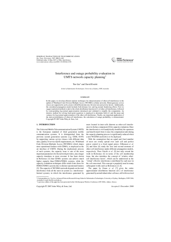3.3. Log-normal approximation of the analytical model Through some trial experiments, the normal probability plot in Figure 1 demonstrates comparison between the simulation results of the logarithm of Fy,x and the corresponding normal distribution. In this figure, the closer the dashed line to the solid line, the more similar the distribution between the simulation results and the normal r.v. From the figure, it is shown that the logarithm of majority samples of Fy,x match the normal distribution very well, thus Fy,x can be well approximated by the log-normal distribution, which reduces the problem to determining only the mean and variance of Fy,x . To calculate these two moments of Fy,x , we can fix the number of users in each y class as n̄t and develop the moments of conditional Fy,x (n̄) first. T   E Fy,x (n̄) = y t=1 n̄t · υt ε∗t Rt ∗R υ W+ε ( t t t) T 1−   · E Dy,x y m=1 , (24) n̄m υm ε∗m Rm W+ε∗m Rm υm       2  E Fy,x (n̄)2 = VAR Fy,x (n̄) + E Fy,x (n̄) (25) where the conditional variance is given by T   VAR Fy,x (n̄) = y n̄t t=1 ·  2 υt ε∗t Rt ∗ (W+εt Rt υt )  1− T m=1   · VAR Dy,x 2 y n̄m υm ε∗m Rm W+ε∗m Rm υm (26) Eur. Trans. Telecomms. 2007; 18:651–660 DOI: 10.1002/ett 657 INTERFERENCE AND OUTAGE EVALUATION Then again applying the theorem of total probabilities to characterise the stochastic number of users, the first and second moments of Fy,x are given as:   E Fy,x =   E F2y,x =   P(n̄y )E Fy,x (n̄) (27)   P(n̄y )E Fy,x (n̄)2 (28) n̄y ∈S n̄y ∈S where P(n̄y ) and S are the corresponding user distribution and admissible region in Equations (15) and (17), respectively. And finally the variance of Fy,x can be simply derived from these two moments as:     2  VAR Fy,x = E F2y,x − E Fy,x (29) One thing to be noticed is that during the calculation of moments of D̂y,x ∈ [0, 1], it is hard to compute the derivative of Equation (21) with respect to z directly, therefore we use the following alternative equations instead.   E D̂y,x = = 1 0 − 1 FD̂ (z) dz (30) 0 E  2 D̂y,x  = 1 z 2     2 VAR Iout y,x = N0 ·VAR Fy,x   = E Iother x   VAR Iother = x FD̂′ (z) dz 0 = z2 FD̂ (z) |10 − 2     E Iout y,x = N0 ·E Fy,x (32) (33) Then following the same assumption in Reference [9] that Iout y,x are independent of each other, the other-cell , which comprises the sum of a series of interference Iother x log-normally distributed r.v.s, can also be approximated by a log-normal r.v. with both parameters as: zFD̂′ (z) dz zFD̂ (z) |10 initial zero for all NodeBs. In the next iteration, the new are used to compute d.f. of Iout d.f. of Iother y,x again and then x other other Ix in turn. The d.f. of Ix would finally converge if the relative changes fall below some thresholds. The analysis is exceedingly tedious since again numerous convolutions are required, however, the excellent lognormal approximation of Fy,x suggests that Iother also x follows log-normal distribution [14], which implies that the mean and variance are sufficient to characterise this r.v. The iterative approach mentioned in Reference [9] is applied to as follows. calculate the moments of Iother x are set to zero in the first step, Iout Since Iother y,x is simply x the product of N0 and Fy,x , which in turn follows lognormal distribution as well. The mean and variance can thus be easily determined as: 1 zFD̂ (z) dz (31) 0 Once Fy,x has been characterised, we can analyse the d.f. of other-cell interference by iteratively solving the fixedand Iout point Equations (12) and (13), where Iother y,x are x used to be the stochastic representation of corresponding set variables within. Starting with the desired r.v. Iother x are determined to zero for all NodeBs, the d.f. of Iout y,x for all possible pairs in a two-tier cell rings system by Equation (13). Then, the sum of Iout y,x for all NodeBs according to y = x yields the other-cell interference Iother x Equation (12) and thus the d.f. of Iother are updated from x Copyright © 2007 John Wiley & Sons, Ltd. (34) y=x   E Iout y,x (35) y=x   VAR Iout y,x , Iout Based on these updated moments of Iother x y,x becomes other the product of two log-normal r.v., (N0 + Iy ) and Fy,x , which again can be regarded as a log-normal r.v. in all the following iterations. The multiplication is performed by summing up the corresponding parameters of these lognormal r.v.s = µ µIout y,x σI2out = σ2 y,x N0 +Iother y N0 +Iother y   + µFy,x (36) + σF2 y,x (37) 2 are the median and variance of the r.v. where µX and σX X’s logarithm, which can be calculated from the mean and Eur. Trans. Telecomms. 2007; 18:651–660 DOI: 10.1002/ett 658 T. LIU AND D. EVERITT variance of X as: 2 σX representation as:  VAR[X] +1 = log E[X]2  ωt = (38) ε∗t Rt W + ε∗t Rt υt (41) then σ2 µX = log (E[X]) − X 2 (39) Stx = Iother x can be determined Again the mean and variance of by Equations (34) and (35), with the moments of Iout y,x derived from the inversion of Equations (38) and (39). In the following, Equations (34)–(37) constitute one whole iteration, which would be repeated until the relative change of interested parameters fall below certain thresholds. The mean and variance of other-cell interference can be obtained after convergence. ωt T 1− m=1 nxm υm ωm  Ixother + N0  (42) It can be seen that within a given cell, the received power Stx of each class only differ from each other in ωt . Hence, if the received power of the user class with maximum ωt is less than the threshold, the other classes must also satisfy the requirements. Then the outage probability can be rewritten as:    x ∗   Poutage = 1 − Pr max St < S t∈T 4. OUTAGE PROBABILITY ANALYSIS In Reference [7], a QoS indicator called outage probability is introduced for capacity analysis in radio network planning. It is assumed in this work that received power of UEs at all their home NodeBs are controlled at the same level, thus the outage probability is defined as the probability that a UE receives an insufficient SIR, which can be easily translated into a constraint on the total interference at one NodeB. Then the calculation of outage probability reduces to the evaluation of the probability that a compound Poisson r.v. exceeds a certain threshold. However, in our current model, since it is presumed that power control aims to maintain SIR for each UE to be constant, a UE can always satisfy the requirement for acceptable QoS unless the requested transmission power, which is proportional to the received power at NodeB, goes beyond its capability. In UMTS networks where multiple classes are supported, the outage probability is approximately defined as:   Poutage = 1 − Pr S1x < S ∗ , S2x < S ∗ , . . . , STx < S ∗ (40) where S ∗ represents a certain received power threshold and Stx is given in Equation (7). With certain traffic class, the parameters such as ε∗t and Rt are fixed values, thus Stx can be characterised as a function of user number nxt and other-cell interference Ixother . If we introduce a class-dependent term ωt for simple Copyright © 2007 John Wiley & Sons, Ltd. = 1 − Pr  St̃x ∗ < S , t̃ : max |ωt | t∈T  (43) Based on the Poisson d.f. for r.v. nxt and acquired log-normal d.f. for Ixother from the previous section, the following analysis is quite straightforward. We have   Pr St̃x < S ∗     T   x   1− nm υ m ω m     m=1 other ∗ <S = Pr Ix − N0   ωt̃       = P (n̄x ) n̄x ∈S     T   xυ ω   1 − n̄   m m m   m=1 other ∗ − N0 · Pr Ix <S   ωt̃       (44) where the notation n̄x , S and P(n̄x ) can be referred to Equations (15)–(17). Under some user allocations, the right hand of the above inequality might be less than zero, in which cases the probability of this summand component simply takes zero since the other-cell interference is always positive. When the Eur. Trans. Telecomms. 2007; 18:651–660 DOI: 10.1002/ett 659 INTERFERENCE AND OUTAGE EVALUATION      T   x   1− n̄m υm ωm         ∗  m=1 other Pr ln Ix < ln S − N0     ωt̃           ln  S∗     = Q       T 1− m=1 n̄xm υm ωm  ωt̃ σI     − N0   − µI           8 7 6 5 4 3 6 8 10 12 14 16 Mean number of UEs per cell (45) where Q(x) is the function given in Equation (21). Hence, together with the parameters µI and σI of othercell interference derived in the previous section, the outage probability in a certain cell can be finally characterised. 5. NUMERICAL RESULTS We consider an area with two-tier hexagonal cell rings surrounding one cell, thus 19 NodeBs in total. Three service classes are assumed in the UMTS system, which are voice users with R1 = 12.2 kbps, ε∗1 = 5.5 dB, low-rate data users with R2 = 28.8 kbps, ε∗2 = 4.0 dB and high-rate data users with R3 = 64 kbps, ε∗3 = 3.5 dB, respectively. The ratio for the number of users of these three classes is 75% : 20% : 5%. The system chip rate W = 3.84 MHz, and background thermal noise N0 = −108 dBm. The activity factor υt are assumed to be 1 for all classes and the PLE γ takes the value of 4. The validation of the analytical model can be performed by Monte-Carlo simulation described above, where the user patterns are generated randomly according to a spatial homogeneous Poisson process, followed by solving a set of linear equations to get the other-cell interference for each NodeB. However, to avoid the border effect due to less neighbours for the cells located at the border, only the sample values at the central cell are counted. Figures 2 and 3 illustrate the comparison of mean and standard deviation between numerical results from Copyright © 2007 John Wiley & Sons, Ltd. Analytical Simulation 9 2 18 20 Figure 2. Comparison of mean other-cell interference. analytical model and simulation results with different average number of users per cell. From the figures, we can see the mean values from both models match quite well, while the standard deviations show slightly greater discrepancy. The reason for this is explained in Reference [9], which is due to the mutual independence out made during the iterative calculation. assumption of Iy,x It impacts on the variance computation and thus underestimates the standard deviation of I other with high loads. The analytical and simulation results of logarithm outage probability Poutage with assumed maximum received power −12 2.6 Std. dev. of other−cell interference [mW]  −12 x 10 10 Mean of other−cell interference [mW] right hand expression is larger than zero, natural logarithm can be applied on both sides. Because ln Ixother follows standard Gaussian distribution with known parameters µI and σI , the probability inside the summand component is actually the tail of Gaussian distribution x 10 Analytical Simulation 2.4 2.2 2 1.8 1.6 1.4 1.2 1 0.8 6 8 10 12 14 16 Mean number of UEs per cell 18 20 Figure 3. Comparison of standard deviation of other-cell interference. Eur. Trans. Telecomms. 2007; 18:651–660 DOI: 10.1002/ett 660 T. LIU AND D. EVERITT mechanisms, each of them results in different othercell interference. Thus, our future work is to provide analytical and approximation models with the incoming traffic regulated by various CAC algorithms. Moreover, the system behaviour in the downlink, or inclusion of packet access data type, are also some interesting topics which remain to be studied. 0 −0.5 Analytical Simulation Log outage probability −1 −1.5 −2 −2.5 ACKNOWLEDGMENTS −3 The authors would like to thank the Smart Internet CRC, Australia for supporting this work as well as to Dr Dirk Staehle and Mr Andreas Mäder for constant fruitful discussions. −3.5 −4 −4.5 10 12 14 16 Mean number of UEs per cell 18 20 Figure 4. Analytical and simulation results for logarithm outage probability. S ∗ = −119 dBm and same user distribution are illustrated in Figure 4. Again, it can be seen that the suggested analytical approximation model can estimate the outage probability excellently. 6. CONCLUSION In this paper, we have presented a purely analytical model for the characterisation of other-cell interference in UMTS networks with log-normal shadowing effects, which is crucial for capacity evaluation during network planning. In theory, the distribution function of othercell interference can be computed based on solving fixedpoint equations iteratively where many convolutions may be involved. A log-normal approximation model is then suggested and verified so that the calculation can be simplified significantly. Finally, one important metric for network capacity planning, outage probability, is introduced and its derivation is demonstrated with fully analytically characterised other-cell interference. In this work, the system behaviour is evaluated under only the simplest CAC scheme. However, in practice, there are many different CAC mechanisms, such as various power-based and number-based CAC. Since the number of active users in the system is controlled by these CAC Copyright © 2007 John Wiley & Sons, Ltd. REFERENCES 1. Gilhousen KS, Jacobs IM, Padovani R, Viterbi AJ, Weaver LA, Wheatley CE. On the capacity of a cellular CDMA system. IEEE Transactions on Vehicular Technology 1991; 40(2):303–312. 2. Everitt D. Traffic engineering of the radio interface for cellular mobile networks. Proceedings of IEEE 1994; 82(9):1371–1382. 3. Holma H, Toskala A. WCDMA for UMTS—radio Access for Third Generation Mobile Communications. John Wiley: Chichester, 2000. 4. Kim KI. CDMA cellular engineering issues. IEEE Transactions on Vehicular Technology 1993;42(3):345–350. 5. Viterbi AJ, Viterbi AM, Zehavi E. Other-cell interference in cellular power-controlled CDMA. IEEE Transactions on Communications 1994; 42(2/3/4):1501–1504. 6. Viterbi AM, Viterbi AJ. Erlang capacity of a power controlled CDMA system. IEEE Journal on Selected Areas in Communications 1993; 11(6):892–900. 7. Evans JS, Everitt D. On the teletraffic capacity of CDMA cellular networks. IEEE Transactions on Vehicular Technology 1999; 48(1):153–165. 8. Karmani G, Sivarajan KN. Capacity evaluation for CDMA cellular systems. In Proceedings of IEEE INFOCOM 2001, Vol 1, pp. 601– 610. 9. Staehle D, Leibnitz K, Heck K, Schröder B, Weller A, TranGia P. Approximating the othercell interference distribution in inhomogeneous UMTS networks. In Proceedings of IEEE 55th Vehicular Technology Conference 2002, Vol 4, pp. 1640–1644. 10. Kleinrock L. Queueing Systems: Theory, Volume I. John Wiley: New York, 1975. 11. Rappaport TS. Wireless Communications: Principles and Practice Prentice Hall: New Jersey, 2002. 12. Cressie NA. Statistics for Spatial Data John Wiley: New York, 1991. 13. Kelly FP. Loss networks. Annals of Applied Probability 1991; 1(3):319–378. 14. Staehle D, Leibnitz K, Heck K, Schröder B, Tran-Gia P, Weller A. An approximation of othercell interference distributions for UMTS systems using fixed-point equations. Institute of Computer Science, University of Wurzburg, Germany, Research Report 292, January 2002. Eur. Trans. Telecomms. 2007; 18:651–660 DOI: 10.1002/ett