Magnetism in graphene nano-islands
J. Fernández-Rossier1, J. J. Palacios1,2
arXiv:0707.2964v2 [cond-mat.mes-hall] 30 Oct 2007
(1)Departamento de Fı́sica Aplicada, Universidad de Alicante,
San Vicente del Raspeig, Alicante E-03690, Spain.
(2)Instituto de Ciencia de Materiales de Madrid (CSIC), Cantoblanco, Madrid E-28049, Spain.
(Dated: February 1, 2008)
We study the magnetic properties of nanometer-sized graphene structures with triangular and
hexagonal shapes terminated by zigzag edges. We discuss how the shape of the island, the imbalance
in the number of atoms belonging to the two graphene sublattices, the existence of zero-energy states,
and the total and local magnetic moment are intimately related. We consider electronic interactions
both in a mean-field approximation of the one-orbital Hubbard model and with density functional
calculations. Both descriptions yield values for the ground state total spin, S, consistent with Lieb’s
theorem for bipartite lattices. Triangles have a finite S for all sizes whereas hexagons have S = 0
and develop local moments above a critical size of ≈ 1.5 nm.
PACS numbers:
The study of graphene-based field effect devices has
opened a new research venue in nanoelectronics1,2,3,4,5 .
Graphene is a truly two-dimensional zero-gap semiconductor with peculiar transport and magnetotransport
properties, including room temperature Quantum Hall
effect6 , that makes it very different from conventional
semiconductors and metals7 . Progress in the fabrication of graphene-based lower dimensional structures
have been reported both in the form of one-dimensional
ribbons8,9 and zero-dimensional dots2,7,10 . Interestingly,
the electronic properties of graphene change in a nontrivial manner when going to lower dimensions. Ribbons,
for instance, can be either semiconducting with a size dependent gap or metallic8,9 .
The electronic structure of graphene-based nanostructures is expected to be different from bulk graphene
because of surface, or, more properly, edge effects12 .
This is particularly true in the case of structures with
ziz-zag edges which present magnetic properties13,14,15 .
Whereas bulk graphene is a diamagnetic semimetal, simple tight-binding models predict that one-dimensional
ribbons with zigzag edges have two flat bands at the
Fermi energy12,13,16,17,18 , i.e., are paramagnetic metals.
Spin polarized density functional theory (DFT)14 and
mean field13 calculations confirm that these bands are
prone to magnetic instabilities.
The fabrication of graphene nanostructures using topbottom techniques does not permit creating atomically
defined edges to date10 . In contrast, bottom-up processing of graphene nano-islands is very promising19 .
Hexagonal shape nano-islands with well-defined zigzag
edges atop the 0001 surface of Ru have already been
achieved20 . This experimental progress motivates our
study of the electronic structure of graphene nanostructures with various shapes. Graphene quantum dots also
hold the promise of extremely long spin relaxation and
decoherence time because of the very small spin-orbit and
hyperfine coupling in carbon11 .
We have found that, remarkably, both the DFT calculations and the mean field approximation of the single-
band Hubbard model with first-neighbors hopping yield
very similar results in all cases considered. Our mean
field results are in agreement with the predictions of
Lieb’s theorem21 regarding the total spin S of the exact ground state of the Hubbard model in bipartite lattices. The honeycomb lattice of graphene is formed by
two triangular interpenetrating sublattices, A and B.
Triangular nanostructures have more atoms in one sublattice, NA 6= NB ; our mean field calculations consistently predict that the total spin of the ground state is
2S = NA − NB and that is mainly localized on the edges.
This could have been anticipated from Hund’s rule and
the appearance, in the non-interacting model, of NA −NB
degenerate states with strictly zero energy. Hexagonal
nanostructures, for which NA = NB , result in S = 0
ground states even when interactions are turned on. A
value of S = 0 does not preclude, however, an interesting
magnetic behavior. In fact, we predict a quantum phase
transition for hexagons: Whereas small ones are paramagnetic, large ones are compensated ferrimagnets, both
with S = 0.
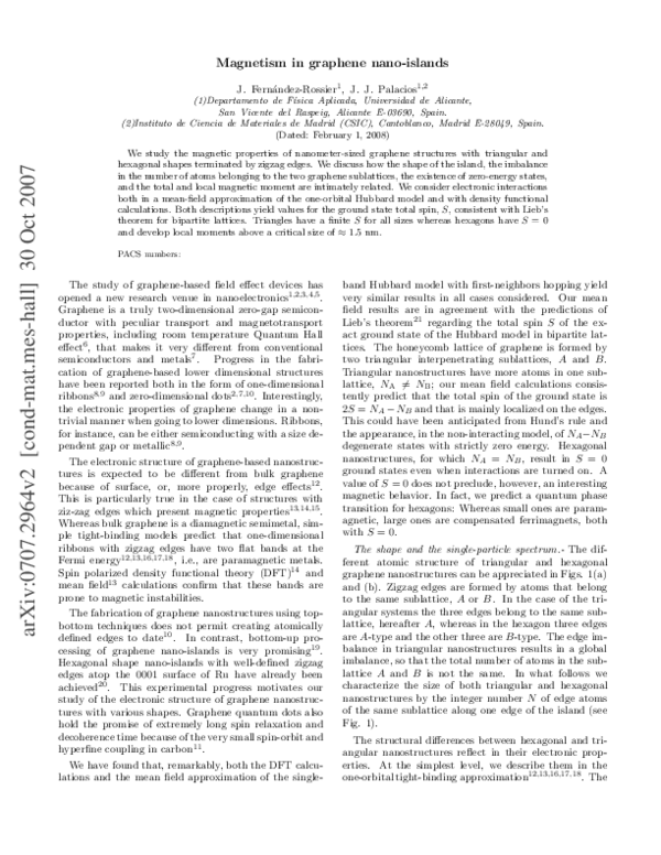
The shape and the single-particle spectrum.- The different atomic structure of triangular and hexagonal
graphene nanostructures can be appreciated in Figs. 1(a)
and (b). Zigzag edges are formed by atoms that belong
to the same sublattice, A or B. In the case of the triangular systems the three edges belong to the same sublattice, hereafter A, whereas in the hexagon three edges
are A-type and the other three are B-type. The edge imbalance in triangular nanostructures results in a global
imbalance, so that the total number of atoms in the sublattice A and B is not the same. In what follows we
characterize the size of both triangular and hexagonal
nanostructures by the integer number N of edge atoms
of the same sublattice along one edge of the island (see
Fig. 1).
The structural differences between hexagonal and triangular nanostructures reflect in their electronic properties. At the simplest level, we describe them in the
one-orbital tight-binding approximation12,13,16,17,18 . The
�2
FIG. 1: (Color online). (a) and (b) Atomic structure of
the triangular and hexagonal graphene islands. (c),(d) Single
particle spectra for the N = 8 triangle (left) and hexagon
(right) (e),(f) Sublattice resolved edge content (eq. 1) and
sublattice polarization (eq. 2)
model Hamiltonian H0 is totally defined by the positions
of the atoms and the first-neighbour hopping parameter
t, which we take equal to 2.5 eV. We set the on-site energies for all the carbon atoms equal to zero. We assume
that the edge atoms are pasivated, so that there are no
dangling bonds. In Figs. 1(c) and (d) we show the (low
energy) spectra corresponding to a triangle (left) and a
hexagon (right) with edge size N = 8. If the system is
charge neutral the relevant electronic states, corresponding to the highest occupied and lowest unoccupied molecular orbitals (HOMOs and LUMOs) are around E = 0.
The most striking difference between the spectra of the
triangle and the hexagon is the existence of a cluster of
zero-energy states in the case of the triangle. A sufficient condition to have NZ states with strict zero energy
in graphene structures is to have a sub-lattice imbalance
NZ = NA − NB . In the case of graphene islands with
triangle shape (see Fig. 1), the sublattice imbalance satisfies NA − NB = N − 1.
In order to quantify the edge/bulk character of the single particle eigenstates φn (I), we define their sub-lattice
resolved edge content:
X
Wη (n) =
|φn (I)|2
(1)
I∈η,edge
where η = A, B and I runs over the Nη atoms. We also
define the sublattice polarization
X
X
L(n) =
|φn (I)|2 −
|φn (I)|2
(2)
I∈A
I∈B
Both in the case of the triangle [Fig. 1 (e)] and the
hexagon [Fig. 1 (f)] states have a predominant edge
character close to the Dirac point (E = 0), but, again,
there are some differences. In the triangle, the zero energy states have a full sublattice polarization L = 1 and
their edge content can reach almost 1. In the case of the
hexagon there is a perfect AB symmetry (L = 0.5) and
the edge content does not go above 0.8.
Electron-electron interactions.- The manifold of 2NZ
zero energy states, including the spin, of the triangle is
half-filled. Electronic repulsions determine which of the
2NZ spin configurations has the the lowest energy. If
Hund’s rule operates in this system, the ground state of
triangular graphene nanostructures (or any other sublattice unbalanced graphene systems, for that matter)
should have a maximal magnetic moment 2S = NZ . In
contrast, the single-particle spectra of hexagons features
some dispersion, which acts against interaction induced
spin polarization. To put this on a quantitative basis,
we have calculated the electronic structure using both a
mean field decoupling of the one-orbital Hubbard model
and DFT calculations in a generalized gradient approximation (GGA) as implemented in the GAUSSIAN03
code22 , using an optimized minimal basis set23 .
FIG. 2: (Color online). Left column: self-consistent energy
spectra for a graphene triangular island with N = 8 (fig 1.a).
Closed (empty) symbols correspond to full (empty) single particle states. Right Column: local magnetization close to one
of the corners of the triangle. Uper row: DFT calculations.
Lower Row: mean field calculations with the Hubbard model.
Magnetization arrows are plotted horizontally for the sake of
clarity
In the mean field approximation for the Hubbard
model we solve iteratively the Hamiltonian
X
H = H0 + U
nI↑ hnI↓ i + nI↓ hnI↑ i,
(3)
I
where H0 is the single particle Hamiltonian described
above and hnIσ i is the statistical expectation value of
�3
the spin-resolved density on atom I, obtained using the
eigenvectors of H. This mean field decoupling can describe spontaneous symmetry breaking along a chosen
axis. The results shown here were obtained fixing N↑
and N↓ , with N↑ + N↓ equal to the number of carbon
atoms in the structure. This permits to compare with
DFT calculations where one typically fixes N↑ − N↓ .
A self-consistent solution of H is characterized by the
n −n
spin density: mI ≡ I,↑ 2 I,↓ , and
P a single particle spectrum ǫn,σ . The total spin S = I mI obviously satisfies
N −N
S = ↑2 ↓.
Uncompensated lattices: Triangles.- In Fig. 2 we show
the spectrum and the spin density for a N = 8 triangle.
Upper panels correspond to DFT results with hydrogen
passivation of the edge atoms. The results in the lower
panel correspond to the mean field results for the Hubbard model. In both cases we have verified that the solutions with N↑ − N↓ = NZ = 7 have lower ground state
energy than solutions with different value of 2S. The
typical energy differences are above 0.5 eV. We choose
the value of U such that the HOMO-LUMO gap in the
majority spectrum is the same. In the case shown in Fig.
2 this corresponds to U = 3.85 eV. Notice that the mean
field and DFT spectrum have very similar structure in
the neighbourhood of EF . Interactions open a spin gap
in the single-particle zero-energy manifold, resulting in
maximal spin polarization of those states. The magnetization density of both calculations is also very similar:
The A atoms on the edge are copolarized positively (right
arrows) and their B neighbour atoms are copolarized negatively. The net total spin is mostly sitting on the edge
and the local magnetization goes to zero in the center of
the island. Using the same procedure as above to fix U ,
we find that its value decreases as the size of the islands
increase. The values of U so obtained are always below
the critical value U ≃ 2.2t ≃ 5.5eV above which infinite
graphene would become antiferromagnetic13,24 .
These results indicate that the Hubbard model captures the low-energy physics of graphene triangular nanoislands. One can conclude that next-to-nearest neighbor
hopping, long-range Coulomb interactions, and correlations, as included in the DFT calculations, have a minor
effect on the low energy sector. Importantly, the basic
features of the mean field solutions, like the structure of
the spectrum, the total spin of the ground state and the
magnetization density, are very robust with respect to
the value of U . We have found very similar results for
triangles with N between 5 and 30. The solution that
minimizes the ground state energy always satisfies
2S = N↑ − N↓ = NA − NB = NZ = N − 1.
(4)
Our mean field Hubbard model and DFT results are
in agreement with the Lieb theorem that states that the
spin S of the ground state of a Hubbard model in a bipartite lattice satisfies the relation 2S = NA − NB 21 .
If the Hubbard model with first-neighbors hopping and
constant U can be applied to graphene-based structures
of arbitrary shape, the theorem permits to predict the
spin of the ground state by simple counting of the sublattice imbalance. The fact that the number of strict
zero energy states NZ equals to NA − NB provides a simple picture of how the magnetization comes about: Spin
polarization results from Hund’s rule and the absence of
kinetic energy penalty in sublattice unbalanced graphene
structures.
Compensated lattices: Hexagons.- In the case of balanced structures Lieb’s theorem predicts that they have
S = 0. This is compatible with a locally unpolarized
state, but also with locally polarized solutions with antiferromagnetic correlations. In these cases, calculations
are necessary to obtain the local magnetization density.
In the case of hexagons there is a competition between
the dispersion of the single-particle spectra and interactions. Dispersion occurs because of the hybridization of
states that otherwise would lie in a single sublattice close
to the edge. These states overlap in the inner region and
close to the vertices and hybridize through hopping in H0 .
Smaller nanostructures feature larger hybridization and
are less prone to develop magnetic order. In the case of
hexagons we expect a critical size above which exchange
interactions take over and the edges magnetize. This is
indeed what we have obtained from our mean field calculations.
The local magnetization mI for the N = 8 hexagon
with U = 2.5eV is shown in the right panel of figure 3.
The local magnetic moments lie mainly on the edges. We
quantify the formation of local moments in compensated
structures by the sublattice resolved average magnetic
moment on the edge atoms
P′
I∈η mI
hmη iedge =
(5)
3N
where η = A, B and the sum runs over the 3N edge atoms
of the η sublattice in the hexagon. For a given value of
U , there is a critical value of N below which this quantity is zero. In Fig. 3a we plot hmη iedge as a function of
N for three different values of U . We always find that
hmA iedge = −hmB iedge . This panel also shows how the
critical size depends on U . When sweeping U in a rather
wide range (U = 1.5 to U = 3.5 eV) the largest possible
paramagnetic hexagon goes from 7 to 4. We have also
estimated the critical size with the help of DFT calculations and found that the largest paramagnetic hexagon
corresponds to N = 8, which is consistent with the mean
field Hubbard results for small U = 1.5eV.
Final remarks and conclusions.- We have seen how the
magnetic properties of graphene nanostructures are intimately related to the sublattice imbalance NA − NB
in agreement with Lieb’s theorem21 . This is related to
previous work on vacancies in graphene25 . As a consequence of Lieb’s theorem a single vacancy results in
the formation of a local moment with S = 1/2 and the
sign of the spin coupling between two single atom vacancies would depend on whether or not they belong to the
same sub-lattice26 . The correlation between sublattice
and sign of the exchange interaction is also seen in our re-
�4
electron transport in systems with spin polarization and
without magnetic anisotropy28. The controlled addition
of single electrons to other nanomagnetic structures, like
magnetic semiconductor quantum dots29 , afford the electrical control of their magnetic properties. This deserves
further attention in the case of magnetic graphene nanoislands.
FIG. 3: (Color online). (a) Sublattice resolved average magnetic moment (eq. (5)) as a function of N for 3 values of U.
(b) Magnetization density for U = 2.5eV and N = 8. Arrows
are plotted vertically for the sake of clarity
sults for triangular and hexagonal nanoislands: Moments
in the same sublattice couple ferromagnetically whereas
moments in different sublattice couple antiferromagnetically. Indirect exchange interaction in graphene follows
the same rule27 .
Nanomagnets show remanence and hysteresys because
of magnetic anisotropy, which originates in the spin-orbit
interaction, very small in graphene. Therefore, the direc~ , of graphene
tion of the spontaneous magnetization, M
nano-islands will fluctutate in the absence of an applied
magnetic field. At zero field, the detection of magnetism
~ |, the modshould rely on properties that depend on |M
ulus of the magnetization vector. An example of this is
the quasiparticle density of states, as probed with single
1
2
3
4
5
6
7
8
9
10
11
12
13
14
15
K. S. Novoselov et al., Science306, 666 (2004)
J. Scott-Bunch et al. Nanoletters 5 287 (2005)
K. S. Novoselov et al., Nature 438, 197 (2005).
Y. Zhang et al., Nature 438, 201 (2005).
C. Berger et al., Science 312, 1191 (2006)
K. S. Novoselov et al. Science 315, 1379 (2007)
A. Geim, K. Novoselov, Nature Materials 6,183 (2007)
Z. Chen et al., cond-mat/0701599.
M. Y. Han, et al., ,Phys. Rev. Lett. 98, 206805 (2007)
B. Ozyilmaz et al. cond-mat/0705.3044
B. Trauzettel et al. Nature Physics 3, 192 (2007)
K. Nakada et al.,Phys. Rev. B54, 17954 (1996)
M. Fujita et al., J. Phys. Soc. Jpn., 65, 1920 (1996)
Y.-W. Son, M. L. Cohen, and S. G. Louie, Nature 444,
347 (2006) Y.-W. Son, M. L. Cohen, and S. G. Louie Phys.
Rev. Lett. 97, 216803 (2006). O. Hod et al., Nano Letters
7, 2295 (2007).
K. Wakabayashi, M. Sigrist, M. Fujita, J. Phys. Soc. Jpn.
In conclusion, we have studied the emergence of magnetism in graphene nano-islands with well-defined zigzag
edges. Our DFT calculations suggest that the magnetic structure of the ground state of graphene nanoislands can be described with a simple Hubbard model.
Ground states with finite spin S appear in structures in
which the number of atoms of one of the sublattices is
larger than the other, NA > NB , like triangular islands.
The single particle spectrum of these structures features
NZ = NA − NB states with strictly zero energy, localized in the A sublattice, which yield a magnetic ground
B
state with finite magnetic moment S = NA −N
when
2
interactions are included, both in a mean field Hubbard
model and with DFT calculations. Compensated structures (NA = NB ) like hexagons have S = 0. However,
they develop spontaneous sublattice magnetization above
a critical size. All our results are nicely consistent with
Lieb’s theorem21 and complement the theorem in the case
of S = 0 ground states.
Note added: Upon the completion of this work we have
been aware of a related work by E. Ezawa30, in the singleparticle approximation, and De-en Jiang et al. and O.
Hod et al. doing DFT calculations31 .
We acknowledge useful discussions with F. Guinea,
B. Wunch, R. Miranda and L. Brey.
This work
has been financially supported by MEC-Spain (Grants
FIS200402356 and Ramon y Cajal Program), by Generalitat Valenciana (Accomp07-054), by Consolider
CSD2007-0010 and, in part, by FEDER funds.
16
17
18
19
20
21
22
23
24
25
26
27
67, 2089 (1998)
M. Ezawa, Phys. Rev. B 73, 045432 (2006).
L. Brey and H. Fertig, Phys. Rev. B73, 235411(2006)
F. Munoz-Rojas et al. , Phys. Rev. B. 74, 195417 (2006)
J. Wu, W. Pisula, and K. Mullen, Chem. Rev., 107, 718
(2007)
A. L. Vázquez de Parga et al. cond-mat/0708.0360
Elliott H. Lieb Phys. Rev. Lett. 62, 1201 (1989)
M.J.Frisch,et. al. , Gaussian 03, Revision B.01, Gaussian,
Inc., Pittsburgh PA, 2003.
M. M. Hurley et al., J. Chem. Phys. 84, 6840 (1986).
N. Peres, M.A. N. Araujo, D. Bozi Phys. Rev. B 70, 195122
(2004)
M. A. H. Vozmediano et al. Phys. Rev. B 72, 155121 (2005)
H. Kumazaki and D. S. Hirashima, J. Phys. Soc. Jpn 76,
064713 (2007)
S. Saremi, arXiv:cond-mat/0705.0187. L. Brey, H. A. Fertig, S. Das Sarma, Phys. Rev. Lett. 99, 116802 (2007)
�5
28
29
C. Gould et al., Phys. Rev. Lett. 97, 017202 (2006). J.
Fernández-Rossier and R. Aguado, Phys. Rev. Lett. 98,
106805 (2007)
J. Fernández-Rossier, L. Brey, Phys. Rev. Lett. 93, 117201
(2004). Y. Leger et al. Phys. Rev. Lett. 97, 107401 (2006).
30
31
M. Ezawa, cond-mat/07070349
De-en Jiang, B. G. Sumpter, and S. Dai, arXiv:0706.0863.
O. Hod, V. Barone, G. E: Scuseria, cond-mat/0709.0938
�
 Juan Palacios