PRL 101, 026805 (2008) week ending 11 JULY 2008 PHYSICAL REVIEW LETTERS Localized Magnetic States in Graphene Bruno Uchoa,1 Valeri N. Kotov,1 N. M. R. Peres,2 and A. H. Castro Neto1 1 Department of Physics, Boston University, 590 Commonwealth Avenue, Boston, Massachusetts 02215, USA 2 Centro de Fı́sica e Departamento de Fı́sica, Universidade do Minho, P-4710-057, Braga, Portugal (Received 21 February 2008; published 11 July 2008; publisher error corrected 11 July 2008) We examine the conditions necessary for the presence of localized magnetic moments on adatoms with inner shell electrons in graphene. We show that the low density of states at the Dirac point, and the anomalous broadening of the adatom electronic level, lead to the formation of magnetic moments for arbitrarily small local charging energy. As a result, we obtain an anomalous scaling of the boundary separating magnetic and nonmagnetic states. We show that, unlike any other material, the formation of magnetic moments can be controlled by an electric field effect. DOI: 10.1103/PhysRevLett.101.026805 PACS numbers: 73.20.Hb, 73.20.
r, 73.23.
b, 81.05.Uw Graphene, a two-dimensional (2D) allotrope of carbon, has singular spectroscopic and transport properties [1– 4] due to its unusual electronic excitations described in terms of massless, chiral, ‘‘relativistic’’ Dirac fermions [5]. In addition to being a possible testbed for relativistic quantum field theory [6], graphene has a great technological potential due to its structural robustness, allowing extreme miniaturization [7], and a flexible electronic structure that can be controlled by an applied perpendicular electric field [8]. In this Letter we show that graphene also has potentiality for spintronics, that is, independent control of the charge and the spin of the charge carriers [9]. Unlike diluted magnetically semiconductors [10] where the location of the magnetic ions is random and hence unpredictable, adatoms can be positioned in graphene using a scanning tunneling microscope (STM) [11]. Furthermore, as we are going to show, the magnetic properties of adatoms such as size of the magnetic moment and Curie temperatures can be controlled by an external electric field, an effect unparalleled in condensed matter systems. The basic model for the study of magnetic moment formation in metals is the well-known Anderson impurity model [12]. In this model an ion with inner shell electrons with energy
0 hybridizes, via a hopping term of energy V, with a conduction sea of electrons. While the conduction electrons are described by a Fermi liquid with featureless, essentially constant, density of states (DOS), the impurity ion is assumed to be strongly interacting. The Coulomb energy required for double occupancy of an energy level in the ion is given by U. Anderson showed that when
0 is below the Fermi energy  and the energy of the doubly occupied states
0  U is larger than , a magnetic state is possible if U is sufficiently large and/or V sufficiently small. Here we apply the Anderson model to graphene and show that the energy dependence of the DOS leads to anomalous broadening of the adatom level and strongly favors the formation of local magnetic moments. In particular we show that, unlike the case of ordinary metals, this anomalous broadening allows the formation of magnetic states even when
0 is above the Fermi energy at relatively small U. We also find, in contrast with the usual 0031-9007=08=101(2)=026805(4) metallic case, an anomalous scaling of the magnetic boundary separating magnetic and nonmagnetic impurity states. Finally, we establish that the local magnetic moments can be mastered by the application of an external gate voltage, leading to a complete control of the magnetic properties of adatoms in graphene. 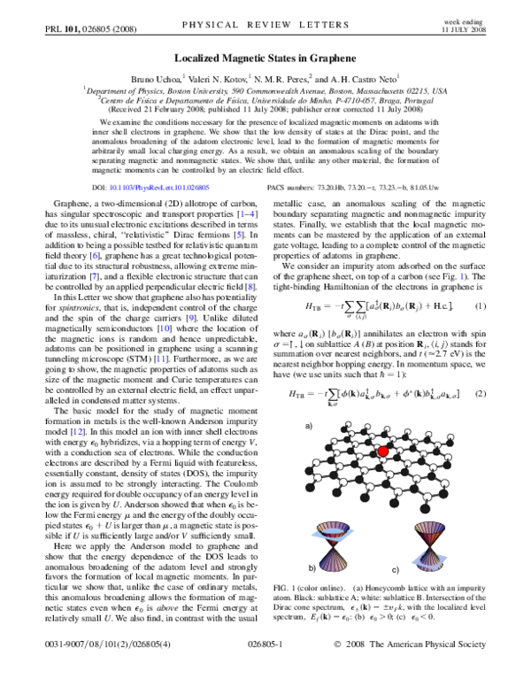We consider an impurity atom adsorbed on the surface of the graphene sheet, on top of a carbon (see Fig. 1). The tight-binding Hamiltonian of the electrons in graphene is XX y HTB 
t a Ri b Rj   H:c:; (1)  hi;ji where a Ri  [b Ri ] annihilates an electron with spin  " , # on sublattice A (B) at position Ri , hi; ji stands for summation over nearest neighbors, and t (2:7 eV) is the nearest neighbor hopping energy. In momentum space, we have (we use units such that @  1): X HTB 
t kayk; bk;   kbyk; ak;  (2) k; a) b) c) FIG. 1 (color online). (a) Honeycomb lattice with an impurity atom. Black: sublattice A; white: sublattice B. Intersection of the Dirac cone spectrum,
k  vF k, with the localized level spectrum, Ef k 
0 : (b)
0 > 0; (c)
0 < 0. 026805-1  2008 The American Physical Society PHYSICAL REVIEW LETTERS PRL 101, 026805 (2008) p


P ~ ^  3=2y, ^ ~ 2  where k  ~ eik  , with ~ 1  ax=2 p


^
3=2y, ^ and ~ 3 
ax^ the nearest neighbor vecax=2 tors. Diagonalization of the Hamiltonian (2) generates two bands,
k  tjkj, which can be linearized around the Dirac points K at the corners of the Brillouin zone:
K  q  vF jqj, where vF  3ta=2 (106 m=s) is the Fermi velocity of the Dirac electrons. The hybridization with the localized orbital of the impurity atom on a given site, say, on sublattice B, is given by P HV  V  fy b 0  H:c:, where f (fy ) annihilates (creates) an electron with spin  " , # at the impurity. In momentum space we have p





X (3) HV  V= Nb  fy bp;  byp; f ; p; where Nb is the number of sites on sublattice B contained in the expanded unit cell of graphene with the impurity. The Hamiltonian of the localized orbital is described P by a single level, Hf 
0  fy f . The electronic correlations in the inner shell states can be described by a Hubbard-like term: HU  Uf"y f" f#y f# . Following Anderson, we use a mean-field decoupling of the interacP tion, HU !  Un
 fy f
Un" n# , where n  hfy f i is the occupation for each of the two spin states. The Hubbard term can be absorbed into the definition of the P local impurity energy, Hf  
 fy f , where
 
0  Un
 is the energy of the localized electrons in a given spin state in the presence of a charging energy U. The formation of a magnetic moment is determined by the occupation of the two spin states at the impurity, n . A localized moment forms whenever n"
n# The determination of n requires the self-consistent calculation of the density of states at the impurity level, ff !, which incorporates the broadening of the impurity level due to hybridization with the bath of electrons in graphene. The occupation of the impurity level is given by Z n  d!ff; !: (4)
1 The Green’s function of f electrons is Gff; t 
ihTf tfy 0i, and its retarded part can be written as GRff; !  !



Rff !  i0 
1 ; (5) where
Rff ! 
V 2 X p G0R bb; p; ! ff; !  2 2 2  G0R bb; p; !  !=!
vF jpj  i0 sign!: In this case (6) becomes (7) 1 j!jD
j!j
1  Z !!

 2  2 !2 (9) where   V 2 =D2 is the dimensionless hybridization. Notice that, unlike the case of impurities in metals, the impurity density of states is not a simple Lorentzian. The impurity DOS (9) is peaked around the quasiparticle pole at
  0 and ! ! 0. We can expand Z! around the singularity at !0 Z
1 !0 
 for !0 ! 0, where we may approximate Z!0  Z
  except for a doublelogarithmic correction that can be safely ignored [13]. The anomalous broadening gives rise to a logarithmic divergence in the ultraviolet when the DOS of the level is integrated in (4),     Z
1 1 jj n 
2  2 

  arctan  

 Z   (10) where Z
   Z and   Z
1  . The term  contains the contribution coming from the cutoff regularization:      W E  1 D
arctan   Z ln  1 ; (11)   DZ
1 
   
 (6) is the self-energy of the f electrons, which is defined in terms of the noninteracting Green’s function of the graphene electrons in a given sublattice, G0bb; p;t 
ihTbp tbyp 0i0 :  2  ! j!
D2 j j!j ln
iV 2 2 D
j!j; D2 !2 D (8) where D is a high-energy cutoff of the order of the graphene bandwidth (D  7 eV). We choose the cutoff D using the Debye prescription, i.e., conservation of the number of states in the Brillouin zone after linearization of the spectrum around the K point. We assume jj D, where band effects related to the exact definition of the cutoff are not important. The real part of
Rff ! defines the quasiparticle residue
1 Z !  1  V 2 =D2  lnjD2
!2 j=!2  of the f electrons, while the imaginary part gives the broadening of the localized level due to the hybridization. As expected, the anomalous character of the problem is explicitly manifested in the linear dependence of the broadening with the energy, which is proportional to the electronic DOS in graphene. Furthermore, notice that Z! vanishes at ! ! 0. Replacing Eq. (8) into Eq. (5) gives the density of states of the localized level, ff; ! 
1=ImGRff; !: where
Rff !  V 2 =Nb  week ending 11 JULY 2008  sign, and q















































2 2 2 E  

Z
1     ; q















































2 2 2 W  DZ
1  
   D  : (12) (13) In Fig. 2 we show the boundary between magnetic and nonmagnetic impurity states as a function of the parameters x  D=U and y  

0 =U. Notice that the magnetic boundary is not symmetric between the cases where the impurity is above (
0 > 0) or below (
0 < 0 026805-2 the Dirac point. Moreover, unlike the metallic problem [12] the boundary is not symmetric around y  0:5. This reflects the particle-hole symmetry breaking due to the presence of the localized level. In the case where
0 > 0 [see Fig. 2(a)], the magnetic boundary crosses the line y  0, and the level magnetizes even when the impurity is above the Fermi energy. This is understood by the fact that the hybridization leads to a large broadening of the impurity level density of states (with a tail that decays like 1=!) that crosses the Fermi energy even when the bare level energy is above it. In the opposite case of
0 < 0 a similar effect occurs with the crossing of the magnetic boundary along the y  1 line, something that also does not occur in ordinary metals [14]. This implies even when the energy of the doubly occupied state is below the Fermi level (
0  U < ), because of the large broadening, the impurity magnetizes if U is not too large or too small. The up turn close to y  1 and x 1 in the
0 < 0 case only reflects that in this limit (U,  
0 , for finite
0 ) the physics of the Dirac points is irrelevant and we recover the usual Anderson model in ordinary metals, where the transition curve approaches the point x  0, y  1 from below [12]. This picture is physically consistent with a renormalization group calculation at fixed   0 [15]. The dependence of the scaling of the magnetic boundary with
0 and  (see Fig. 2) shows that the size of the magnetic region grows as j
0 j approaches the energy of the Dirac points. In this situation the DOS around the localized level is suppressed, favoring the formation of a local magnetic moment. In particular, in the limit where the level is nearly at the Dirac point (j
0 j ! 0, the level nearly decouples from the bath and the impurity can magnetize in principle for any small finite charging energy U. On the other hand, the magnetic region shrinks in the y direction 1 a) 1.5 b) non-magnetic 0.5 1 as the hybridization parameter  grows (see Fig. 2). In the limit of  ! 0 and U finite a local magnetic moment forms whenever 0 < y < 1, as in the case of an impurity in a metal. The application of a potential Vg through an electric field via a back gate [1] shifts the chemical potential  and moves the magnetic state of the impurity in the vertical direction (y) in Fig. 2. We assume that x  D=U does not change much with applied voltage, even with screening coming from a finite Fermi energy. Hence, the magnetization of the impurity can in principle be turned on and off, depending only on the gate voltage applied to graphene. This is better illustrated by looking at the behavior of the impurity magnetic susceptibility. In the presence of a field, the energy of the impurity spin states changes to
 
0
B B  Un
 . In the zero field limit, P the magnetic susceptibility of the impurity,  B  dn =dBB0 (B is the Bohr magneton, and B is an applied magnetic field), can be calculated straightforwardly from Eq. (10): 
2B
 X dn 1
U dn d

 :
 dn d
 1
U2 dn "# d

 d
 1 1 a) 0.5 0 0 χ ( µB2 102 ) -0.5 εo < 0 5 x = ∆D/U 10 0 0 5 c) 0.5 0.5 0 non-magnetic εo > 0 10 0 b) d) 10 0.1 5 0 0.1 x = ∆D/U 0.2 µ (eV) FIG. 2 (color online). Boundary between magnetic and nonmagnetic impurity states in the scaling variables x and y for
0 > 0 (a) and
0 < 0 (b). Circles: j
0 j=D  0:029, V=D  V=D  0:14; 0:14; squares:
0 =D  0:043 and triangles:j
0 j=D  0:029, V=D  0:03. The upturn close to y  1 and x ! 0 on panel (b) is not visible in this scale when V is very small (triangles). See details in the text. (14) In the lower panels of Fig. 3 we show  for
0  0:2 eV, V 1 eV, and D 7 eV, for different values of x. The corresponding magnetization line for this set of parameters is defined by the solid curve with black circles in Fig. 2(a). While the impurity remains nonmagnetic for any y at x  11 (U 40 meV), as shown in Fig. 2(a), the impurity state already crosses the magnetic boundary twice for x  5, where U is nearly twice as large. In this case, a large magnetic moment of 0:5 B forms below the energy of the level, at  0:18 eV [Fig. 3(a) and 3(b)]. At x  0:45 (U  1 eV), the local moment exists for very large  1 eV, and a strong and uniform magnetic moment of 0:9B forms in almost the whole magnetic region [see Fig. 3(c)]. A similar qualitative behavior for the magnetization occurs when
0 < 0 [Fig. 3(c) and 3(d)]. As U becomes large (>1 eV), the magnetic transition becomes very sharp. For
0 0:5 eV and V  1 eV, the impurity can magnetize for U * 0:1 eV. While the local nσ y = (µ- εo)/U week ending 11 JULY 2008 PHYSICAL REVIEW LETTERS PRL 101, 026805 (2008) 0.3 0 -0.5 0 0.5 1 1.5 µ (eV) FIG. 3 (color online). n" , n# , and  for j
0 j=D  0:029 and V=D  0:14 (D 7 eV). Left panels: x  11 (dashed curves), and x  5 (solid curves). The impurity magnetizes inside the bubble (n"
n# . The vertical line marks the position of the level,
0  0:2 eV. On the right:
0  0:2 eV (solid curve) and
0 
0:2 eV (dashed curve) at x  0:45. 026805-3 PHYSICAL REVIEW LETTERS PRL 101, 026805 (2008) Aff(µ) 300 a) 120 200 80 100 40 0 0.1 0.2 0.3 0 b) 0 0.5 1 µ (eV) µ (eV) FIG. 4 (color online). Spectral function (in units of 1/eV) of the f electrons at the Fermi energy  for j
0 j=D  0:029 and V=D  0:14 (D 7 eV). (a) x  11 (solid curve) and x  5 (dashed curve) for
0 > 0 (see Fig. 2). (b) x  0:45 for
0 > 0 (solid curve) and
0 < 0 (dashed curve). charging energy U for transition metals in a metallic matrix is of the order of 5–10 eV [16], in graphene, where the effective hybridization can be large due to the linear increase of the DOS, the critical U for magnetization of the impurity can be much smaller. Hence, transition elements and molecules that usually do not magnetize when introduced in ordinary metals can actually become magnetic in graphene [17,18]. In order to show that the spectroscopic functions of the magnetic impurities can also be controlled by electric field effect we show, in Fig. 4, the spectral function of the localized electrons P calculated at the Fermi energy: Aff !    2  ff; . The solid line in Fig. 4(a) is a nonmagnetic resonance in a situation where the impurity state does not cross the magnetic boundary of the scaling diagram by changing y () for some fixed x. In the other curves of Fig. 4, the spectral weight splits between two peaks located around the magnetic transitions, near 
0 and
0  U (see Fig. 3). The dependence of the impurity density of states with , and hence with gate bias, allows for the identification of the formation of local moments through ordinary transport measurements. For finite , the hybridization of the itinerant electrons with the localized level renormalizes the charge scattering channels and hence the carrier conductivity,   2e2 jj , where
1 is the impurity scattering rate. Second order perturbation theory gives [16]
1

1 0 / n0 V 2 Aff ; interaction is purely ferromagnetic due to the vanishing of the Fermi wave vector, kF  =vF [24]. However, at finite bias voltage the RKKY interactions display 2kF oscillations decaying like 1=r3 [25] that can couple the magnetic moments ferromagnetically or antiferromagnetically depending on the position and geometry of the adatom lattice (that can be conveniently chosen using a STM). Hence, by changing the bias voltage a variety of different magnetic phases can emerge. In conclusion, we have examined the conditions under which a transition metal adatom on graphene can form a local magnetic moment. We find that due to the anomalous broadening of the adatom local electronic states, moment formation is much easier in graphene. Furthermore, the magnetic properties of adatoms can be controlled by an electric field effect allowing for the possibility of using graphene in spintronics. We thank V. M. Pereira, J. M. B. Lopes dos Santos, A. Polkovnikov, and S. W. Tsai for helpful discussions. N. M. R. P. acknowledges financial support from POCI 2010 via Project No. PTDC/FIS/64404/2006. B. U. acknowledges CNPq, Brazil, for support under Grant No. 201007/2005-3. [1] [2] [3] [4] [5] [6] [7] [8] [9] [10] [11] [12] [13] [14] (15) where
1 is the scattering rate of the electrons in the 0 absence of impurities and n0 is the impurity concentration. In the limit of very large U, however, the scattering is dominated by the spin flip channels in the Kondo regime [19–23]. When
0 is located in the experimental range accessible by the application of a gate voltage
0:3 to 0.3 eV [1], the shape of the dip in the conductivity produced by the impurity scattering can indicate not only the position of the energy level but also the presence of local magnetic moments (notice that the nonmagnetic resonance in the spectral function is quite symmetric). In the presence of a finite density of magnetic moments a macroscopic magnetic state can egress due to the RKKY interaction between them. At the Dirac point (  0) the week ending 11 JULY 2008 [15] [16] [17] [18] [19] [20] [21] [22] [23] [24] [25] 026805-4 K. S. Novoselov et al., Science 306, 666 (2004). K. S. Novoselov et al., Nature (London) 438, 197 (2005). Y. Zhang et al., Nature (London) 438, 201 (2005). A. K. Geim and K. S. Novoselov, Nat. Mater. 6, 183 (2007). A. H. Castro Neto et al., arXiv:0709.1163. A. H. Castro Neto et al., Phys. World 19, 33 (2006). L. A. Ponomarenko et al., Science 320, 356 (2008). E. V. Castro et al., Phys. Rev. Lett. 99, 216802 (2007). S. A. Wolf et al., Science 294, 1488 (2001). A. H. MacDonald et al., Nat. Mater. 4, 195 (2005). D. M. Eigler et al., Nature (London) 344, 524 (1990). P. W. Anderson, Phys. Rev. 124, 41 (1961). The approximation on Z! leads to a deviation of 1% from the exact numerical calculation in the scaling diagram. A single crossing at y  1 was found for an Anderson impurity in a chiral Luttinger liquid, P. Phillips and N. Sandler, Phys. Rev. B 53, R468 (1996). L. Fritz and M. Vojta, Phys. Rev. B 70, 214427 (2004). G. D. Mahan, Many Particle Physics (Plenum, New York, 2000), 3rd ed. D. M. Duffy and J. A. Blackman, Phys. Rev. B 58, 7443 (1998). O. Leenaerts et al., Phys. Rev. B 77, 125416 (2008). D. Withoff and E. Fradkin, Phys. Rev. Lett. 64, 1835 (1990). G.-M. Zhang et al., Phys. Rev. Lett. 86, 704 (2001). M. Hentschel and F. Guinea, Phys. Rev. B 76, 115407 (2007). B. Dora and P. Thalmeier, Phys. Rev. B 76, 115435 (2007). K. Sengupta and G. Baskaran, Phys. Rev. B 77, 045417 (2008). M. A. H. Vozmediano et al., Phys. Rev. B 72, 155121 (2005). V. V. Cheianov et al., Phys. Rev. Lett. 97, 226801 (2006).