MARINE ECOLOGY PROGRESS SERIES Mar Ecol Prog Ser Vol. 393: 235–246, 2009 doi: 10.3354/meps08222 Contribution to the Theme Section ‘Marine ecosystems, climate and phenology: impacts on top predators’ Published October 30 OPEN ACCESS Climate change and phenological responses of two seabird species breeding in the high-Arctic Børge Moe1, 2,*, Lech Stempniewicz3, Dariusz Jakubas3, Frédéric Angelier4, 5, Olivier Chastel4, Frode Dinessen6, Geir W. Gabrielsen7, Frank Hanssen8, Nina J. Karnovsky9, Bernt Rønning1, Jorg Welcker7, Katarzyna Wojczulanis-Jakubas3, Claus Bech1 1 Department of Biology, Norwegian University of Science and Technology (NTNU), 7491 Trondheim, Norway 2 Norwegian Institute for Nature Research (NINA), Division of Arctic Ecology, 9296 Tromsø, Norway 3 Department of Vertebrate Ecology and Zoology, University of Gdansk, al. Legionów 9, 80-441 Gdansk, Poland 4 Centre d’Etudes Biologiques de Chizé, Centre National de la Recherche Scientifique, 79360 Villiers en Bois, France 5 Smithsonian Migratory Bird Center, Smithsonian Institution, Washington, DC 20008, USA 6 Norwegian Meteorological Institute, 9293 Tromsø, Norway 7 Norwegian Polar Institute, 9296 Tromsø, Norway 8 Norwegian Institute for Nature Research (NINA), 7485 Trondheim, Norway 9 Department of Biology, Pomona College, Claremont, California 91711, USA ABSTRACT: The timing of breeding is a life-history trait that can greatly affect fitness, because successful reproduction depends on the match between the food requirements for raising young and the seasonal peak in food availability. We analysed phenology (hatch dates) in relation to climate change for 2 seabird species breeding in the high-Arctic, little auks Alle alle and black-legged kittiwakes Rissa tridactyla, for the periods 1963–2008 and 1970–2008, respectively. We show that spring climate has changed during the study period, with a strong increase in both air temperature (TEMP) and sea surface temperature (SST) and a decrease in sea ice concentration. Little auks showed a trend for earlier breeding over the study period, while kittiwakes showed a non-significant trend for later breeding, demonstrating different phenological responses in these 2 species. Little auks and kittiwakes adjusted their timing of breeding to different environmental signals. Spring TEMP was the best predictor of little auk phenology, with a significant negative effect. Spring SST was the strongest predictor of kittiwake phenology, with a non-significant negative effect. Spring sea ice concentration and the North Atlantic Oscillation (NAO) winter index had a low relative variable importance. Furthermore, in kittiwakes, years with late breeding were associated with low clutch size and mean annual breeding success, indicating poor investment and food availability. This study identifies some spring environmental factors important for regulating the timing of breeding in the high-Arctic, most likely through effects on snow cover limiting access to nest sites and the development of the polar marine food web. It remains to be investigated whether environmental factors are reliable predictors of marine prey phenology, and whether the decision to start breeding is constrained by food availability. KEY WORDS: Phenology · Climate change · Seabirds · Match-mismatch · Svalbard · Sea ice · Temperature · Timing of breeding Resale or republication not permitted without written consent of the publisher Some of the strongest evidence for the effects of climate change on organisms comes from studies of phenology (e.g. Stenseth et al. 2002, Walther et al. 2002). Phenology is the timing of seasonal activities of animals and plants, and long-term trends for changes in arrival dates and breeding dates of birds have been regarded as ‘fingerprints’ of the ongoing climate change (Parmesan & Yohe 2003, Root et al. 2003). *Email: borge.moe@nina.no © Inter-Research 2009 · www.int-res.com INTRODUCTION 236 Mar Ecol Prog Ser 393: 235–246, 2009 In regions where food availability is highly seasonal, reproduction is only possible during a short time period, usually during the spring and summer. The timing of the peak in food availability varies between years. Hence, the timing of breeding is crucial in order to match the energy requirements of breeding to the actual food availability (the temporal match-mismatch concept; Cushing 1990, Edwards & Richardson 2004, Frederiksen et al. 2004, Durant et al. 2005). Thus, the timing of breeding is among the key factors for successful reproduction in birds (Dunn 2004, Reed et al. 2009). The decision to start breeding is under endocrine control, and the hormone levels involved in this control are influenced by a combination of fixed (photoperiod) and variable environmental cues (climatic factors, food availability; Wingfield 1983, Gwinner 1986). Birds experience variable environmental cues on different spatial and temporal scales, and evidence suggests that birds use these cues in optimal decisions on when to initiate breeding (e.g. Frederiksen et al. 2004). The decision is done before the peak in food availability occurs, so optimal decisions are possible if the environmental cues are reliable predictors of the peak in food availability (Visser & Both 2005). In addition, initiation of breeding could be constrained by the food availability during the prebreeding period that is needed for investment in eggs. In extreme cases, egg production relies on endogenous reserves built up before and during migration (‘capital breeders’; Drent & Daan 1980). However, most birds produce their eggs from resources acquired at the breeding grounds (‘income breeders’; Drent & Daan 1980). The Arctic region is currently undergoing a dramatic climate change, with a 2-fold higher increase in temperature compared to the global increase, a trend that is expected to continue (Kattsov et al. 2005, IPCC 2007). Advancement in the onset of spring is already evident, with the timing of snow melt becoming 15 d earlier over the last decade in Greenland (Høye et al. 2007). Furthermore, sea ice extent has decreased linearly by 3 to 9% per decade in the Arctic Ocean (Serreze et al. 2007), with substantial effects on polar marine ecosystems (Gaston et al. 2003, Moline et al. 2008). The development of the polar marine food web on which seabirds depend is closely linked to the timing of removal of sea ice and the warming and stratification of the surface waters to allow for a spring bloom. Consequently, there is a need to assess the effects of climate change on Arctic seabirds. With some exceptions, however, there are very few published long-term studies on breeding phenology from the Arctic. In the Canadian Arctic, years with low sea ice cover and early sea ice break-up were related to early breeding of Brünnich’s guillemots Uria lomvia (Gaston et al. 2005a). While low sea ice cover negatively affected breeding success of the lowArctic population, breeding success of the high-Arctic population was positively affected by early sea ice break-up (Gaston et al. 2005a). In East Antarctica, a decrease in sea ice cover and an increase in the length of the sea ice season were associated with a trend for later breeding of adelie penguins Pygoscelis adeliae and cape petrels Daption capense (Barbraud & Weimerskirch 2006). These studies suggest that sea ice affects seabird breeding phenology and breeding success in high-latitude regions. They also underline the fact that climate change has not affected all parts of the polar regions to the same extent or in the same direction (Vaughan et al. 2001). 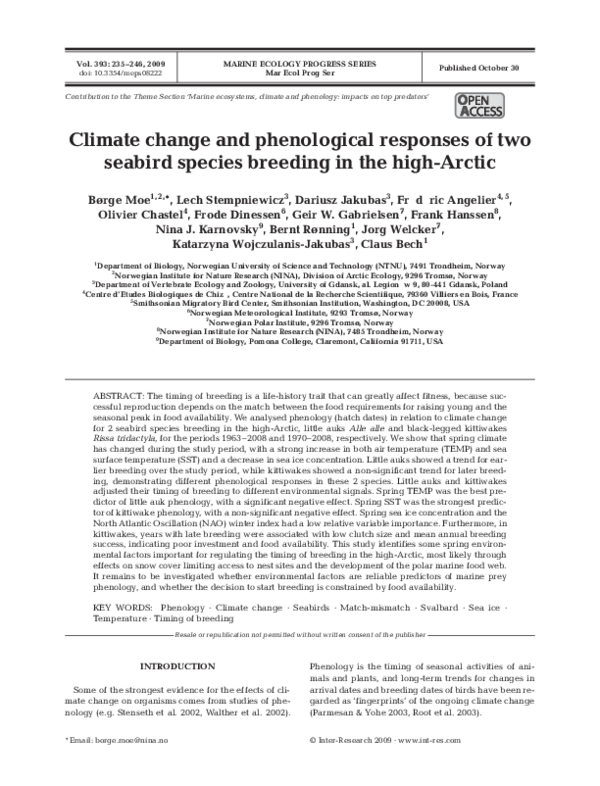In the present study, we analysed long-term data on breeding phenology of 2 high-Arctic breeding seabirds, black-legged kittiwakes Rissa tridactyla (hereafter ‘kittiwakes’) and little auks Alle alle, breeding at Ny-Ålesund and Hornsund, respectively, on the western coast of Svalbard (Fig. 1). These data cover the periods 1970–2008 and 1963–2008 for kittiwakes and little auks, respectively, and offer a great opportunity to detect long-term changes in the timing of breeding in relation to climate change in the high-Arctic and to test whether environmental conditions at different scales explain the variability in the timing of breeding. Migratory seabirds may use the winter conditions to initiate the spring migration (Frederiksen et al. 2004), and we used the North Atlantic Oscillation index (NAO) as a large-scale proxy for winter conditions. Our study populations spend the winter in the Northwest Atlantic Ocean, close to Greenland according to ring recoveries (Bakken et al. 2003). If they use the winter conditions to initiate the spring migration, and this in turn affects the timing of breeding, we expected NAO to affect the breeding phenology of both species. When the seabirds arrive at the breeding grounds in spring, they may use local environmental cues or food availability to further adjust the timing of breeding (Frederiksen et al. 2004). Both of these birds are ‘income breeders’. Just after arrival at their breeding grounds, kittiwakes and little auks feed at different trophic levels (Karnovsky et al. 2008). In the early part of the breeding season, little auks are primarily zooplanktivorous: they feed at a low trophic level on copepods (e.g. Karnovsky et al. 2003, 2008). Little auks from West Greenland have been known to arrive at their breeding grounds just when copepods such as Calanus hyperboreus rise to the surface waters to feed on the spring phytoplankton bloom that is linked to stratification of the water column (Karnovsky & Hunt 2002). In contrast, kittiwakes feed at a higher trophic level on fish, amphipods and krill (Hop et al. 2002, Karnovsky et al. 2008). We used spring sea surface temperature (SST) and sea ice concentration (ICE) to represent the environmental conditions in the foraging areas at sea, and we expected both species to breed earlier in years Moe et al.: Seabird breeding phenology in the high-Arctic 60°W 30° 0° 30° 60°E 70°N 30°E 80°N Ny-Ålesund 78° Longyearbyen Hornsund 0 100 76° 10°E 200 Km 20° Fig. 1. Study area on Spitsbergen, Svalbard. Kittiwakes were studied at Ny-Ålesund and little auks in Hornsund, and large white circles indicate the 2 study colonies. Meteorological stations (small black circles) in Ny-Ålesund, Longyearbyen and Hornsund provided data on air temperature. The boxes show the areas from which data on sea surface temperatures (SST) and sea ice concentrations (ICE) were obtained (see ‘Materials and methods: Environmental parameters’) with low ICE and high SST (Gaston et al. 2005a, Barbraud & Weimerskirch 2006). The ground-nesting little auks breed in a rocky slope that is covered by snow during spring. Hence, access to the nests is only available when the snow cover has melted sufficiently. However, snow does not block access to nests for the cliff-nesting kittiwakes. By using spring air temperature (TEMP) as an indicator of timing of snow melt, we expected TEMP to affect little auk but not kittiwake phenology. Furthermore, in kittiwakes, we also tested the hypothesis that inter-annual variation in the timing of breeding would be related to fecundity and breeding success. MATERIALS AND METHODS Breeding phenology. Data on median hatch date of little auks was obtained in a large colony (~10 000 breeding pairs) at the Ariekammen slopes (77° 00’ N, 237 15° 33’ E) in Hornsund, Svalbard (Fig. 1). Published (Stempniewicz 2001, Harding et al. 2004) and unpublished data on median hatch date were obtained for 18 years in the period 1963–2008 (1963–65, 1974–75, 1980, 1983–84, 1986–87 and 2001–08). Hatch date was determined by regular visual inspections of 17 to 261 nests in the same area of the colony for all years, except for one. In 2003, hatch date was back-calculated from the median date of fledging (departure of 857 fledglings during 14 nights of observation that covered the whole fledging period; Wojczulanis et al. 2005) and the length of the nesting period (27 d; Stempniewicz 1981). Median hatch dates of kittiwakes were obtained in the colony Krykkjefjellet (78° 54’ N, 12° 13’ E) in Kongsfjorden, 6 km from Ny-Ålesund in Svalbard (Fig. 1). Since 2002, we included a second colony (Irgensfjellet; 79° 00’ N, 12° 07’ E). It is located only 10 km away from the other and comprises approximately the same number of nests. This was done to maintain robust sample sizes after a substantial decline in the population size (during 1997–2003), and to maintain high precision in the measure of hatch date. Published (Mehlum 2006) and unpublished data were obtained for 18 years in the period 1970–2008 (1970–71, 1982–85 and 1997–2008). The median hatch dates for 2004–2008 were determined by regular visual inspections of ~180 nests, and in 1997–2000 we inspected ~100 nests. In 2002 and 2003, we used hatch dates of chicks (2002, N = 18; 2003, N = 5) that were hatched in an artificial egg incubator (A90, J. Hemel; T = 37.5–38°C, relative humidity 55–75%), because breeding was extremely late and the hatching occurred when the field workers were not present. The chicks originated from eggs that were collected in the colony, insulated with wool and brought to the laboratory in Ny-Ålesund within 1 h upon collection. Median hatch dates for 1970–1971, 1982–1985 and 2001 were determined from counts of hatched eggshells under the bird cliff in the same colony (Krykkjefjellet) by Mehlum (2006). We did a methodological study and observed hatch dates in the nests and counted hatched eggshells under the same nests (covering 112 nests). This showed that counts of hatched eggshells produced a 0.5 d later median hatch date, compared to direct observations in the nests. Accordingly, we adjusted the hatch dates obtained from Mehlum (2006) by –0.5 d. Breeding success. For kittiwakes, data on clutch size and a measure of breeding success (number of chicks >12 d old per active nest) were obtained for all years in the period 1997–2008 (51 to 139 active nests), except for 2001. Data on breeding success of little auks were only available for a few years, and consequently were not analysed. Environmental parameters. We used the NAO as a large-scale measure of winter conditions and 3 local measures of spring conditions (SST, ICE and TEMP). 238 Mar Ecol Prog Ser 393: 235–246, 2009 Monthly NAO indices, standardised by the 1950–2000 base period monthly means and SD, were obtained from the National Oceanic and Atmospheric Administration (NOAA; www.cpc.ncep.noaa.gov) to produce a winter index (NAOW, averaged over December to March). Measures averaged for April–May were used for local spring conditions, because both kittiwakes and little auks return to the breeding grounds in Svalbard in April, and egg-laying occurs in June. Data on TEMP (°C) were obtained from the weather stations in Ny-Ålesund and Longyearbyen (Norwegian Meteorological Institute, DNMI) and Hornsund (Polish Polar Station Hornsund; Fig. 1). Data on TEMP from Ny-Ålesund were used in the analyses of kittiwake phenology. In analyses of little auk phenology, we used data on TEMP from Hornsund for the period 1979–2007 and estimated data on TEMP for Hornsund for the period 1963–1979. By using the estimates from a linear regression, we made a reliable estimate of TEMP for Hornsund from TEMP Longyearbyen (TEMP Hornsund = –0.36 [± 0.27] + 0.794 [± 0.037] × TEMP Longyearbyen), because these measures were highly correlated (1979–2008, N = 30, r = 0.97, p < 0.0005). The conclusions drawn in this study did not differ if we entirely used TEMP Longyearbyen to represent TEMP Hornsund. Furthermore, we expected the timing of snow melt to influence the breeding phenology of little auks. Data on snow depth or snow cover, however, do not exist for the appropriate time scales, so we used TEMP as a proxy for the timing of snow melt. ICE (%) was extracted with the software ArcGIS Arcinfo (9.2) from sea ice maps. DNMI has produced daily maps (1979–2008) and weekly maps (1963–1979) by manual interpretation of satellite data and in situ observations. Sea ice maps were unavailable for May 1964 from Hornsund. We therefore estimated ICE May from ICE April (ICE May = 0.59 × ICE April – 0.127, F1,41 = 25.5, p < 0.001). Maps were unavailable for April and May in 1964 and 1965 for Ny-Ålesund. The sea ice cover at the western coast of Spitsbergen typically consists of different types of drift ice, ranging from ‘very close drift ice’ to ‘open water’, with 90–100% and 0–10% ice concentrations, respectively. Data on sea temperature at 5 m depth were used as SST (°C). These data were obtained from the CartonGiese SODA v2.0.2-4 database (Carton & Giese 2008) via the IRI/LDEO Climate Data Library (http://iridl. ldeo.columbia.edu). The SST data from Carton-Giese SODA v2.0.2-4 covered the whole study period except for the last year. SST for 2008 was therefore estimated from SST obtained from Reyn_Smith OIv2 (Reynolds et al. 2002) via the IRI/LDEO Climate Data Library. We simply multiplied the SST from 2007 by the 2008/2007 SST ratio from Reyn_Smith OIv2. We used ICE data from the 1° box bounded by 78– 79° N and 10–11°E for the kittiwakes breeding at NyÅlesund (Fig. 1) and by 76–77° N and 15–16° E for the little auks breeding in Hornsund (Fig. 1). The sea ice is more extensive close to the coast compared to farther west, so data from these areas are the best to reflect the sea ice conditions. We used SST data from the 2° boxes bounded by 78–79° N and 8–10° E and by 76–77° N and 13–15° E for the kittiwakes and the little auks, respectively (Fig. 1). We chose these boxes to cover a relatively large area that included both the shelf and the area to the west of the shelf break. From GPStracking, we know that this geographical sector correspond well to the foraging areas during the pre-breeding period for the kittiwakes breeding at Ny-Ålesund (O. Chastel unpubl. data). We do not have knowledge about the foraging grounds of the little auks during the pre-breeding period. However, the chosen area corresponds well to the foraging areas during the breeding period (Karnovsky et al. 2003). Statistical analyses. Linear regressions and Pearson moment-product correlations were used to test for temporal trends in environmental factors and timing of breeding. We followed the approach by Frederiksen et al. (2004) to test how environmental variables affected breeding phenology. We entered TEMP, ICE, SST, NAOW and YEAR as predictor variables in multiple linear models where median hatch date was the response. We used diagnostic plots (QQ, residuals versus fitted, residuals versus leverage) to assess whether the data sufficiently met the assumptions of the linear model. We fitted 32 models for each species and included no interactions. The selection of the best models was based on Akaike’s Information Criterion adjusted for small samples size (AICc; Burnham & Anderson 2002). To avoid models with very limited support, we selected a redefined set of candidate models with ΔAICc < 4 and calculated AICc weights. AICc weight is the likelihood of the model given the data and the set of candidate models, and evidence ratios summarise this for each predictor variable. Thus, AICc weight and evidence ratio represent the relative importance of a model and a predictor variable, respectively. Evidence ratios >10 indicate moderately strong support (Lukacs et al. 2007, Frederiksen et al. 2008). The effect of each environmental variable on breeding phenology was estimated using model-averaged estimates that were calculated using AICc weights according to Burnham & Anderson (2002). Hence, the effects were adjusted for model selection uncertainty. It was important to include YEAR in these analyses, because some of the environmental variables showed a linear trend over time (Fig. 2, Table A1 in Appendix 1). Other predictor variables also correlated with each other (Table A1), so we carefully compared models Moe et al.: Seabird breeding phenology in the high-Arctic 239 The analyses could potentially be affected by the fact that different methods had been used to obtain hatch dates. For kittiwakes, data from 2002 and 2003 were special because hatch dates were obtained from eggs in incubators, and because these years were extremely late and poor. For little auks, data from 2003 was special because hatch date was back-calculated from fledging dates. We therefore performed reanalyses to test how environmental variables affected breeding phenology when these years were excluded. However, the results from these reanalyses did not change the conclusions drawn from the full analyses with all years included. The statistical analyses were performed with the software R 2.6.0 (R Development Core Team 2007). The seabird and environmental data used in this study are given in Appendix 1, Table A2. RESULTS Fig 2. (A) Air temperature (TEMP), (B) sea ice concentration (ICE) and (C) sea surface temperature (SST) at (d) Ny-Ålesund, (s) Hornsund and ( ) Longyearbyen as a function of year. (D) North Atlantic Oscillation winter index (NAOW) as a function of year. The data on TEMP are from the periods 1963–2008, 1969–2008 and 1979–2008 from Longyearbyen, Ny-Ålesund and Hornsund, respectively. Regression lines indicate significant linear relationships. (A) TEMP Longyearbyen = –194.3 (± 42.4) + 0.094 (± 0.021) × year; TEMP Ny-Ålesund = –196.6 (± 53.3) + 0.096 (± 0.027) × year; TEMP Hornsund = –213.3 (± 76.2) + 0.104 (± 0.038) × year, (B) ICE Ny-Ålesund = 958.8 (± 333.7) – 0.475 (± 0.168) × year; ICE Hornsund = 1775.8 (± 617.4) – 0.873 (± 0.310) × year; (C) SST Ny-Ålesund = –57.8 (±18.2) + 0.031 (± 0.009) × year; SST Hornsund = –63.1 (±19.0) + 0.034 (± 0.010) × year; (D) NAOW = –50.7 (±13.0) + 0.026 (± 0.007) × year containing only 1 variable to those of multiple variables. The SEs of the estimates were not severely inflated when multiple variables were included in the same models, so the conclusions drawn from these analyses are not assumed to be influenced by problems related to multiple collinearity. Spring TEMP increased in Svalbard over the study period (1963–2008), with TEMP becoming 0.9 (± 0.2)°C warmer per decade in Longyearbyen (F1,44 = 19.4, p < 0.001, Fig. 2A). The strongest increase in TEMP took place during the later part of this period, with an increase of 0.47 (± 0.18)°C per year from 1997 to 2008 (F1,10 = 6.9, p = 0.03, Fig. 2A). The increase in TEMP was similar for Hornsund and Ny-Ålesund (Fig. 2A). This trend was accompanied by a decrease in spring ICE and by an increase in spring SST. During the whole study period, the decrease in ICE was significant for Ny-Ålesund (F1,42 = 8.0, p = 0.007, Fig. 2B), but not entirely for Hornsund (F1,44 = 2.3, p = 0.14, Fig. 2B). During the last 30 yr, however, it was significant for both locations (1978–2008, F1,29 > 5.5, p < 0.02, Fig. 2B). SST increased significantly over the study period for Ny-Ålesund (F1,44 = 11.2, p = 0.002, Fig. 2C) and Hornsund (F1,44 = 12.1, p = 0.001, Fig. 2C). The NAOW also increased significantly during the study period (F1,44 = 15.3, p < 0.001, Fig. 2D). Little auks showed a significant trend for earlier breeding (F1,16 = 4.5, p = 0.05, Fig. 3); median hatch date became 4.5 (± 2.1) d earlier over the study period. The kittiwakes showed a trend for later hatching, but it was not significant (F1,16 = 1.7, p = 0.21, Fig. 3). For the years with data from both species, there was no correlation between the median hatch dates of kittiwakes and little auks (r = 0.06, df = 8, p = 0.86), indicating that the 2 species have shown different phenological responses over time. Different environmental factors were related to the breeding phenology of little auks than kittiwakes (Tables 1 & 2). The best models were TEMP for little auks and SST+ICE for kittiwakes (Table 1), with coefficients of determination (R2) of 0.40 and 0.30, respec- Mar Ecol Prog Ser 393: 235–246, 2009 240 Table 2. Alle alle and Rissa tridactyla. Effects of environmental variables on breeding phenology of little auks and kittiwakes. Effects are model-averaged slope estimates derived from the models in Table 1. Variables are ranked according to the evidence ratio (ER), which reflects their relative importance. Shown are unconditional SEs and 95% confidence intervals. ER was calculated as the summed Akaike weights of all models including the variable divided by the summed weight of models not including the variable. ER > 10 indicates moderate to strong support. Units are °C for TEMP and SST and % for ICE. See ‘Materials and methods: Environmental parameters’ for an explanation of model parameters Fig 3. Alle alle and Rissa tridactyla. Median hatch dates in July of little auks (open circles) and kittiwakes (filled circles) breeding in Svalbard, as a function of year (kittiwakes, 18 yr, 1970–2008; little auks, 18 yr, 1963–2008). The regression line represents a significant linear trend for earlier breeding of little auks; hatch date = 217.2 (± 93.7) – 0.100 (± 0.047) × year Table 1. Alle alle and Rissa tridactyla. Rank of linear models explaining breeding phenology of little auks and kittiwakes based on Akaike’s Information Criterion corrected for small sample size (AICc). k is the number of parameters, and w is the Akaike weight calculated from the set of models with ΔAICc < 4. See ‘Materials and methods: Environmental parameters’ for an explanation of model parameters Rank Model k ΔAICc w Little auks 1 2 3 4 5 6 7 8 TEMP TEMP, ICE TEMP, SST TEMP, YEAR TEMP, NAOW TEMP, ICE, SST TEMP, ICE, NAOW ICE 2 3 3 3 3 4 4 2 0.0 0.1 2.6 3.3 3.4 3.5 3.9 3.9 0.33 0.31 0.09 0.06 0.06 0.06 0.05 0.05 Kittiwakes 1 2 3 4 5 6 7 8 9 SST, ICE SST, ICE, YEAR SST, YEAR intercept only SST YEAR YEAR, NAOW SST, ICE, NAOW SST, ICE, TEMP 3 4 3 1 2 2 3 4 4 0.0 1.9 2.2 2.3 2.7 3.3 3.6 3.9 3.9 0.34 0.13 0.11 0.11 0.09 0.06 0.06 0.05 0.05 tively. TEMP was the best predictor of little auk phenology, while SST was the best predictor of kittiwake phenology (Tables 1 & 2). High TEMP was associated with early breeding of little auks, while high SST was associated with early breeding of kittiwakes (Table 2). For little auks, TEMP had an evidence ratio that indicated moderately strong support relative to the other predictor variables (Table 2), and the confidence inter- Variable Effect SE 95% CI ER Little auks TEMP ICE SST NAOW YEAR –1.02 0.04 –0.09 0.02 –0.001 0.45 0.06 0.22 0.14 0.005 –1.89, –0.14 –0.07, 0.16 –0.51, 0.34 –0.26, 0.30 –0.010, 0.008 19.0 0.9 0.2 0.1 0.1 Kittiwakes SST ICE YEAR NAOW TEMP –3.54 –0.13 0.05 –0.20 –0.003 2.66 0.14 0.08 0.57 0.032 –8.75, 1.67 –0.39, 0.14 –0.11, 0.22 –1.33, 0.92 –0.066, 0.060 3.3 1.3 0.6 0.1 0.1 val of the model-averaged slope estimate did not overlap with 0 (Table 2). Hence, TEMP seemed to have an important negative relationship with breeding phenology of little auks. For kittiwakes, however, the modelaveraged slope estimate for SST overlapped slightly with 0 and the evidence ratio was relatively low (Table 2), and we cannot conclude firmly about the effect or the relative importance of the variable. Although ranked second best, ICE had low relative variable importance, and the effects were highly uncertain (Table 2). Furthermore, NAOW and YEAR had the lowest evidence ratios, and the model-averaged slope estimates were very close to 0 (Table 2). Notably, the significant correlation between YEAR and little auk phenology (Fig. 3) disappeared when TEMP was included in the models (Table 2). Hence, it seems likely that the trend for increased spring TEMP (Fig. 2) has caused the trend for earlier breeding of little auks (Fig. 3). In kittiwakes, clutch size (r = –0.84, df = 9, p = 0.001, Fig. 4) and breeding success (r = –0.80, df = 9, p = 0.003, Fig. 4) were negatively correlated to median hatch dates. When breeding success was calculated as the number of chicks per egg laid, instead of the number of chicks per active nest, the negative correlation with phenology was still significant (r = –0.83, df = 9, p = 0.001). Thus, late breeding was associated with low clutch size and poor breeding success (Fig. 4). These relationships, however, were strongly driven by the 2 extremely late years, i.e. 2002 and 2003, and the correlations were not significant when these years were excluded. Moe et al.: Seabird breeding phenology in the high-Arctic Fig. 4. Rissa tridactyla. Mean annual clutch size (filled triangles) and breeding success (number of chicks >12 d old per active nest; open triangles) of kittiwakes in relation to median hatch date (in July) during the breeding seasons 1997–2008 (N = 11, no data on clutch size or breeding success in 2001). Regression lines indicate significant linear relationships DISCUSSION The main findings of this study were that (1) median hatch date of little auks advanced during the study period, while hatch dates of kittiwakes tended to become later (albeit not significantly); (2) spring TEMP was a strong environmental predictor of little auk phenology, while spring SST tended to be an important environmental predictor of kittiwake phenology; and (3) clutch size and breeding success of kittiwakes was negatively related to the timing of breeding. Kittiwakes and little auks thus showed some different phenological responses. Temporal trends in the timing of breeding 241 phenological responses adds to a diverse picture of seabird phenology in polar and temperate regions. Studies have reported trends for earlier (Catharacta maccormicki, Fratercula cirrhata, Sterna paradisaea, Uria lomvia) and later breeding (Daption capense, Fulmarus glacialis, Pygoscelis adeliae, Rissa tridactyla, U. aalge), as well as no detectable trends (Aptenodytes forsteri, Fratercula arctica, Fulmarus glacialis, Pagodroma nivea, Ptychoramphus aleuticus, U. aalge, U. lomvia; e.g. Gjerdrum et al. 2003, Abraham & Sydeman 2004, Durant et al. 2004, Frederiksen et al. 2004, Gaston et al. 2005a, 2009, Barbraud & Weimerskirch 2006, Møller et al. 2006, Wanless et al. 2008, 2009, Reed et al. 2009). This diverse pattern may indicate that the phenology of specific seabird species is regulated by different environmental factors (e.g. Frederiksen et al. 2004, Barbraud & Weimerskirch 2006), or that climate has changed in different degrees or directions in different parts of the world (e.g. Vaughan et al. 2001). Hornsund and Ny-Ålesund are located relatively close (Fig. 1) and are strongly correlated environments (Table 3, Fig. 2), and it is not likely that the different trends are caused by climate change having acted differently on Hornsund and Ny-Ålesund. Rather, we think that the different ecologies of the 2 species have created the different phenological responses. Environmental predictors of seabird phenology TEMP and SST in combination with ICE were the highest ranked models explaining little auk and kittiwake phenology, respectively (Table 1), and TEMP and SST were the variables with the highest relative importance (Table 2). Conditional on the candidate models and the data, this suggests that local environmental factors during spring are the most important predictors of timing of breeding in these 2 high-Arctic populations. Indeed, we think spring TEMP is strongly linked to the timing of snow melt and to the time when ground-nesting little auks can have access to snow- To our knowledge, this is the first little auk study with long-term phenology data and, consequently, the first to detect a trend for earlier breeding. The timing of breeding advanced by 4.5 d during Table 3. Mean and SE of environmental variables (TEMP, SST and ICE) of Ny1963–2008. Another alcid species, Ålesund and Hornsund in April–May of the periods 1963–2008 (SST and ICE) Brünnich’s guillemot, advanced breedand 1979–2008 (TEMP). Shown are the correlations of the environmental variing by 5 d during 1988–2007 in the ables between the 2 locations and a comparison of the means (paired t-test). The Canadian low-Arctic but showed no difference in SST between the locations was reversed if data on SST were obtained closer to the coast trend in the high-Arctic (Gaston et al. 2005a, 2009). The trend for later breeding of kittiwakes, although not signifiNy-Ålesund Hornsund Correlation Paired t-test Mean SE Mean SE N r p t p cant, is in accordance with trends for later breeding of British kittiwake popTEMP –6.5 0.43 –5.7 0.37 30 0.84 < 0.01 –2.3 0.03 ulations (Frederiksen et al. 2004, WanSST 2.9 0.13 3.2 0.14 46 0.71 < 0.01 –2.4 0.02 less et al. 2009). The finding that kittiICE 15.4 2.31 35.6 2.42 44 0.70 < 0.01 –10.5 < 0.01 wakes and little auks showed different 242 Mar Ecol Prog Ser 393: 235–246, 2009 free nest sites in the rock debris colony slope. Unfortunately, we do not have appropriate data on snow cover, but behavioural observations and temperature measurements at Hornsund in 2006 strengthen this interpretation. The little auk colony was constantly occupied by birds in the colony only after the ground temperature and the nest temperature were permanently above 0°C (Fig. 5). The little auks then occupied nests as soon as the snow cover melted sufficiently to allow access to the nests. Therefore, the timing of egglaying seemed to be strongly determined by temperature and snow melt in the colony (Fig. 5), consistent with a study on ground-nesting auklets (Aethia pusilia, A. cristatella, Cyclorrhynchus psittacula) in Alaska (Sealy 1975). Effects of spring snow cover and TEMP on phenology have also been reported in other groundnesting bird species in the high-Arctic, such as waders (Calidris alba, C. alpina, Arenaria interpres; Meltofte et al. 2007), greater snow geese Chen caerulescens atlantica (Bêty et al. 2003, Dickey et al. 2008) and pinkfooted geese Anser brachyrhynchus (Madsen et al. 2007). In addition to effects via snow cover, temperature could also directly impose energetic constraints on little auk phenology. Temperatures are often below the Fig. 5. Alle alle. Temperature (°C) in little auk nests (solid line), underground locations in the colony slope (broken line) and ground (measured ~20 cm above flat tundra; thick solid line) as a function of date in 2006. ‘Irregular presence’ means that the colony attendance alternated between periods without any birds and periods with many birds in the colony. ‘Permanent presence’ means that the colony was constantly attended by little auks. The arrow indicates median egg-laying date in 2006, and the box indicates the egg-laying period. Ground temperature was measured 3 times d–1. Temperature was measured every hour in 3 nests and 4 underground locations, and this graph presents the hourly means for these 3 nests and 4 underground locations, respectively. Temperature loggers in the 3 nests were removed on 4 June, i.e. before egg laying occurred thermoneutral zone (TNZ) when they lay eggs (TNZ > 4.5°C, Gabrielsen et al. 1991), and costs of egg production and incubation are elevated under such conditions (Stevenson & Bryant 2000). SST correlated negatively to kittiwake phenology, but we cannot conclude firmly that SST had an effect, because the confidence intervals of the modelaveraged slope estimate slightly overlapped with 0 (Table 2). This is in accordance with studies of kittiwakes (Frederiksen et al. 2004) and tufted puffins Fratercula cirrhata (Gjerdrum et al. 2003) at lower latitudes. Those studies reported significant negative correlations with local SST, but they disappeared when a longer time series was analysed for the kittiwakes (Frederiksen et al. 2004, Wanless et al. 2009) and when all years were included in the tufted puffin data (Gjerdrum et al. 2003). Wanless et al. (2009) reported longterm phenology data for British seabirds, and SST did not correlate significantly to phenology of any of the 11 investigated species. Hence, the effect of SST on seabird phenology seems weak or unclear. Studies from the Arctic and the Antarctic have shown that seabirds breed later in years with more sea ice or a longer sea ice season (Gaston et al. 2005a,b, Barbraud & Weimerskirch 2006). Extensive ICE could force arctic seabirds to forage in more distant waters and make early breeding energetically expensive, and late disappearance of sea ice and development of the polar marine food web could delay the optimal timing of breeding (Moline et al. 2008). However, we did not detect a clear effect of ICE on phenology, as the signs of the model-average slope estimates differed between kittiwakes and little auks and the confidence intervals considerably overlapped with 0 (Table 2). This result is somewhat unexpected, especially for little auks breeding at Hornsund, because the sea ice cover can be rather extensive in this area (Fig. 2B, Table 3). We used NAOW as a large-scale proxy for winter conditions, and detected no effect on phenology (Fig. 2). However, we cannot rule out the possibility that kittiwakes breeding in the high-Arctic assess their winter conditions to adjust the timing of breeding, as reported for kittiwakes, common guillemots Uria aalge, Atlantic puffins Fratercula arctica and razorbills Alca torda breeding in Great Britain (Frederiksen et al. 2004, Wanless et al. 2009). Kittiwakes and little auks are likely to disperse over a large area in the North Atlantic during winter, and the evidence for wintering close to Greenland is sparse (Bakken et al. 2003). Because the correlation between NAO and local climate (e.g. SST) is highly spatially variable, it is not clear how well NAOW captures the winter conditions of kittiwakes and little auks. Our phenological time series covered substantial time periods (1963–2008, 1970–2008, Fig. 3). However, Moe et al.: Seabird breeding phenology in the high-Arctic data were not available for all the years within these periods, and the time series had some substantial gaps (Fig. 3). Complete time series would have provided (1) better precision in the descriptions of the temporal trends in the timing of breeding and (2) more statistical power to detect potential relationships between environmental factors and timing. It is not clear whether kittiwakes and little auks use the environmental cues in optimal decisions on when to initiate breeding. We have no data on phenology of the main prey items of little auks and kittiwakes (copepods versus fish/amphipods/krill). Therefore, we are consequently unable to test whether specific environmental variables are reliable predictors of marine prey phenology (Visser & Both 2005). We do not think TEMP is a direct predictor of marine prey phenology. SST and ICE could be such predictors through their effects on the timing of spring bloom and phenology of phytoplankton and zooplankton (Edwards & Richardson 2004, Scott et al. 2006, Moline et al. 2008). Alternatively, the ability of kittiwakes and little auks to initiate breeding could be constrained by food availability, because they rely on food acquired at the breeding grounds for investment in their eggs. Reed et al. (2009) reported that fish abundance affected phenology of common guillemots in California, but appropriate data to test this for our populations do not exist. Thus, our results are not conclusive on whether breeding phenology is regulated by optimal decisions or constrained by food availability. 243 temperature and SST and the decrease in sea ice concentration are consistent with rapidly advancing spring and timing of snow melt in Greenland (Høye et al. 2007). Thus, further advancements in the timing of breeding could be expected for little auks and other ground-nesting high-Arctic species. A possible consequence of an earlier snow melt is the opening of new breeding grounds at the limits of the species’ range (Jensen et al. 2008), with a displacement of the population towards the colder areas (e.g. Gaston et al. 2005a, Stempniewicz et al. 2007). Although SST tended to have some importance, it is not sufficiently clear how kittiwake phenology is affected by environmental factors to make sound future predictions. We investigated seabird phenology in the high-Arctic in relation to environmental factors. Local environmental factors during spring seem to be stronger predictors than winter conditions, but it is unclear how well the considered variable (NAOW) captures the winter conditions. It remains to be investigated whether specific environmental variables are reliable predictors of marine prey phenology, whether the initiation of breeding is constrained by food availability, and how well seabirds are able to match the peak in food availability in the high-Arctic. Since phenology, abundance and composition of marine prey species may change as climate changes (Edwards & Richardson 2004, Wassmann et al. 2006), this is important for understanding the fitness consequences of future climate change. Acknowledgements. Permission to do field work was granted by the Governor of Svalbard. We thank all field workers and the staff at the Polish Polar Station in Hornsund (Institute of Geophysics, Polish Academy of Science), Sverdrup Station (Norwegian Polar Institute) and Rabot Station (Institut PaulEmile Victor) in Ny-Ålesund. We thank D. Puczko for preparation of meteorological data from Hornsund and C. Barbraud, I. Herfindal, H. Sandvik and BJ. Bårdsen for comments on the manuscript. M. Frederiksen and 3 anonymous referees provided constructive comments that improved this manuscript. C.B., B.M., B.R., J.W. and G.W.G. were supported by the Norwegian Research Council and by ‘Arktisstipend’. L.S., D.J. and K.W. were supported by the Polish Ministry of Science and Higher Education. O.C. and F.A. were supported by the Institut Paul-Emile Victor and by CNRS/Région PoitouCharentes. N.K. was supported by the National Science Foundation. Breeding success and phenology Kittiwake clutch size and breeding success were significantly negatively related to the timing of breeding (Fig. 4), indicating poor investment and poor food availability in years with very late breeding. The same relationship has been found for other Arctic kittiwake populations in Alaska (Murphy et al. 1991) and Canada (Gaston et al. 2005b), but not at lower latitudes in Scotland (Frederiksen et al. 2004). The Arctic summer is very short, so this relationship could indicate that a late peak in food availability is associated with a very short peak or a very low peak in food availability, and that the low breeding success achieved in the late LITERATURE CITED years is the best possible in these years. However, we do not know how well kittiwakes are able to match the ➤ Abraham CL, Sydeman WJ (2004) Ocean climate, euphausipeak in food availability. ids and auklet nesting: inter-annual trends and variation CONCLUSIONS AND FUTURE CONSIDERATIONS The spring climate is currently undergoing big changes in this part of Svalbard. The increase in air ➤ in phenology, diet and growth of a planktivorous seabird, Ptychoramphus aleuticus. Mar Ecol Prog Ser 274:235–250 Bakken V, Runde O, Tjørve E (2003) Norsk ringmerkingsatlas, Vol 1. Stavanger Museum, Stavanger Barbraud C, Weimerskirch H (2006) Antarctic birds breed later in response to climate change. Proc Natl Acad Sci USA 103:6248–6251 244 Mar Ecol Prog Ser 393: 235–246, 2009 ➤ Bêty J, Gauthier G, Giroux JF (2003) Body condition, migra- ➤ ➤ ➤ ➤ ➤ ➤ ➤ ➤ ➤ ➤ ➤ ➤ ➤ ➤ ➤ tion, and timing or reproduction in snow geese: a test of the condition-dependent model of optimal clutch size. Am Nat 162:110–121 Burnham KP, Anderson DR (2002) Model selection and multimodel inference. A practical information-theoretic approach. Springer-Verlag, Heidelberg Carton JA, Giese BS (2008) SODA: a reanalysis of ocean climate. Mon Weather Rev 136:2999–3017 Cushing DH (1990) Plankton production and year class strength in fish populations — an update of the match-mismatch hypothesis. Adv Mar Biol 26:249–293 Dickey MH, Gauthier G, Cadieux MC (2008) Climatic effects on the breeding phenology and reproductive success of an arctic-nesting goose species. Glob Change Biol 14: 1973–1985 Drent RH, Daan S (1980) The prudent parent: energetic adjustments in avian breeding. Ardea 68:225–252 Dunn P (2004) Breeding dates and reproductive performance. Adv Ecol Res 35:69–87 Durant JM, Anker-Nilssen T, Hjermann DØ, Stenseth NC (2004) Regime shifts in the breeding of an Atlantic puffin population. Ecol Lett 7:388–394 Durant JM, Hjermann DØ, Anker-Nilssen T, Beaugrand G, Mysterud A, Pettorelli N, Stenseth NC (2005) Timing and abundance as key mechanisms affecting trophic interactions in variable environments. Ecol Lett 8:952–958 Edwards M, Richardson AJ (2004) Impact of climate change on marine pelagic phenology and trophic mismatch. Nature 430:881–884 Frederiksen M, Harris MP, Daunt F, Rothery P, Wanless S (2004) Scale-dependent climate signals drive breeding phenology of three seabird species. Glob Change Biol 10: 1214–1221 Frederiksen M, Jensen M, Daunt F, Mavor RA, Wanless S (2008) Differential effects of a local industrial sand lance fishery on seabird breeding performance. Ecol Appl 18: 701–710 Gabrielsen GW, Taylor JRE, Konarzewski M, Mehlum F (1991) Field and laboratory metabolism and thermoregulation in dovekies (Alle alle). Auk 108:71–78 Gaston AJ, Woo K, Hipfner JM (2003) Trends in forage fish populations in northern Hudson Bay since 1981, as determined from the diet of nestling thick-billed murres Uria lomvia. Arctic 56:227–233 Gaston AJ, Gilchrist HG, Hipfner JM (2005a) Climate change, ice conditions and reproduction in an Arctic nesting marine bird: Brünnich’s guillemot (Uria lomvia L.). J Anim Ecol 74:832–841 Gaston AJ, Gilchrist HG, Mallory ML (2005b) Variation in ice conditions has strong effects on the breeding of marine birds at Prince Leopold Island, Nunavut. Ecography 28: 331–344 Gaston AJ, Gilchrist HG, Mallory ML, Smith PA (2009) Changes in seasonal events, peak food availability, and consequent breeding adjustment in a marine bird: a case of progressive mismatching. Condor 111:111–119 Gjerdrum C, Vallee AMJ, St Clair CC, Betram DF, Ryder JL, Blackburn GS (2003) Tufted puffin reproduction reveals ocean climate variability. Proc Natl Acad Sci USA 100: 9377–9382 Gwinner E 1986. Circannual rhythms: endogenous annual clocks in the organization of seasonal processes. Springer, Berlin Harding AMA, Van Pelt TI, Lifjeld JT, Mehlum F (2004) Sex differences in little auk Alle alle parental care: transition from biparental to paternal-only care. Ibis 146:642–651 Hop H, Pearson T, Hegseth EN, Kovacs KM and others (2002) ➤ ➤ ➤ ➤ ➤ ➤ ➤ ➤ ➤ ➤ ➤ ➤ ➤ The marine ecosystem of Kongsfjorden. Polar Res 21: 167–208 Høye TT, Post E, Meltofte H, Schmidt NM, Forchhammer MC (2007) Rapid advancement of spring in the High Arctic. Curr Biol 17:R449–R451 IPCC (2007) Climate change 2007: the physical science basis. Summary for policy makers. Contribution of Working Group I to the Fourth Assessment Report of the Inter-governmental Panel on Climate Change. Cambridge University Press, Cambridge Jensen RA, Madsen J, O’Connell M, Wisz MS, Tommervik H, Mehlum F (2008) Prediction of the distribution of Arcticnesting pink-footed geese under a warmer climate scenario. Glob Change Biol 14:1–10 Karnovsky NJ, Hunt GL Jr (2002) Estimation of carbon flux to dovekies (Alle alle) in the North Water. Deep-Sea Res II 49:5117–5130 Karnovsky NJ, Kwaśniewski S, Wȩs8awski JM, Walkusz W, Beszczyńska-Möller A (2003) Foraging behavior of little auks in a heterogeneous environment. Mar Ecol Prog Ser 253:289–303 Karnovsky NJ, Hobson KA, Iverson S, Hunt GL Jr (2008) Seasonal changes in diets of seabirds in the North Water Polynya: a multiple-indicator approach. Mar Ecol Prog Ser 357:291–299 Kattsov VM, Källén E, Howard C, Christensen J and others (2005) Future climate change: modelling and scenarios for the Arctic. In: Symon C, Arris L, Heal B (eds) Arctic climate impact assessment. Cambridge University Press, Cambridge, p 99–150 Lukacs PM, Thompson WL, Kendall WL, Gould WR, Doherty PF, Burnham KP, Anderson DR (2007) Concern regarding a call for pluralism of information theory and hypothesis testing. J Appl Ecol 44:456–460 Madsen J, Tamstorf M, Klaassen M, Eide N and others (2007) Effects of snow cover on the timing and success of reproduction in high-Arctic pink-footed geese Anser brachyrhynchus. Polar Biol 30:1363–1372 Mehlum F (2006) Co-variation between climate signals and breeding phenology of high-arctic breeding kittiwakes (Rissa tridactyla). Mem Natl Inst Pol Res 59:29–37 Meltofte H, Høye TT, Schmidt NM, Forchhammer MC (2007) Differences in food abundance cause inter-annual variation in the breeding phenology of High Arctic waders. Polar Biol 30:601–606 Moline MA, Karnovsky NJ, Brown Z, Divoky GJ and others (2008) High latitude changes in ice dynamics and their impact on polar marine ecosystems. Ann NY Acad Sci 1134:267–319 Møller AP, Flensted-Jensen E, Mardal W (2006) Rapidly advancing laying date in a seabird and the changing advantage of early reproduction. J Anim Ecol 75: 657–665 Murphy EC, Springer AM, Roseneau DG (1991) High annual variability in reproductive success of kittiwakes (Rissa tridactyla L.) at a colony in western Alaska. J Anim Ecol 60: 515–534 Parmesan C, Yohe G (2003) A globally coherent fingerprint of climate change impacts across natural systems. Nature 421: 37–42 R Development Core Team (2007) R: a language and environment for statistical computing. R Foundation for Statistical Computing, Vienna Reed TE, Warzybok P, Wilson AJ, Bradley RW, Wanless S, Sydeman WJ (2009) Timing is everything: flexible phenology and shifting selection in a colonial seabird. J Anim Ecol 78:376–387 Reynolds RW, Rayner NA, Smith TM, Stokes DC, Wang WQ 245 Moe et al.: Seabird breeding phenology in the high-Arctic ➤ ➤ ➤ ➤ (2002) An improved in situ and satellite SST analysis for climate. J Clim 15:1609–1625 Root TL, Hall KR, Schreider SH, Rosenzweig C, Pounds JA (2003) Fingerprints of global warming on wild animals and plants. Nature 421:57–60 Scott BE, Sharples J, Wanless S, Ross ON, Frederiksen M, Daunt F (2006) The use of biologically meaningful oceanographic indices to separate the effects of climate and fisheries on seabird breeding success. In: Boyd I, Wanless S, Camphusyen CJ (eds) Top predators in marine ecosystems: their role in monitoring and management. Cambridge University Press, Cambridge, p 46–62 Sealy SG (1975) Influence of snow on egg-laying in auklets. Auk 92:528–538 Serreze MC, Holland MM, Stroeve J (2007) Perspectives on the Arctic’s shrinking sea-ice cover. Science 315:1533–1536 Stempniewicz L (1981) Breeding biology of the little auk (Plautus alle) in the Hornsund region, SW Spitsbergen. Acta Ornithol 18:141–165 Stempniewicz L (2001) Little auk Alle alle. BWP update. J Birds Western Palearctic 3:175–201 Stempniewicz L, Blachowlak-Samolyk K, Weslawski JM (2007) Impact of climate change on zooplankton communities, seabird populations and Arctic terrestrial ecosystem — a scenario. Deep-Sea Res II 54:2934–2945 Stenseth NC, Mysterud A, Ottersen G, Hurrell JW, Chan KS, Lima M (2002) Ecological effects of climate fluctuations. Science 297:1292–1296 ➤ Stevenson ➤ ➤ ➤ ➤ ➤ ➤ IR, Bryant DM (2000) Climate change and constraints on breeding. Nature 406:366–367 Vaughan DG, Marshall GJ, Connolley WM, King JC, Mulvaney R (2001) Climate change — devil in the detail. Science 293:1777–1779 Visser M, Both C (2005) Shifts in phenology due to global climate change: the need for a yardstick. Proc R Soc Lond B Biol Sci 272:2561–2569 Walther GR, Post E, Convey P, Menzel A and others (2002) Ecological responses to recent climate change. Nature 416:389–395 Wanless S, Harris MP, Lewis S, Frederiksen M, Murray S (2008) Later breeding in northern gannets in the eastern Atlantic. Mar Ecol Prog Ser 370:263–269 Wanless S, Frederiksen M, Walton J, Harris MP (2009) Longterm changes in breeding phenology at two seabird colonies in the western North Sea. Ibis 151:274–285 Wassmann P, Reigstad M, Haug T, Rudels B and others (2006) Food webs and carbon flux in the Barents Sea. Prog Oceanogr 71:232–287 Wingfield JC (1983) Environmental and endocrine control of avian reproduction: an ecological approach. In: Mikami S, Wada M (eds) Avian endocrinology: environmental and ecological aspects. Japan Science Society Press, Tokyo, and Springer-Verlag, Berlin, p 205–288 Wojczulanis K, Jakubas D, Stempniewicz L (2005) Changes in the glaucous gull predatory pressure on little auks in southwest Spitsbergen. Waterbirds 28:430–435 Appendix 1. Data used in models of phenology for little auks Alle alle and black-legged kittiwakes Rissa tridactyla and of climate change in Svalbard Table A1. Rissa tridactyla and Alle alle. Correlation matrix of predictor variables used in the linear models analysing hatch date in relation to environmental variables (Table 1). Pearson’s product moment correlations are presented with p-values in parentheses. See ‘Materials and methods: Environmental parameters’ for an explanation of model parameters YEAR NAOW TEMP SST Kittiwakes (1970–2008) N = 18 NAOW TEMP SST ICE 0.38 (0.12) 0.47 (0.05) 0.23 (0.36) –0.39 (0.11) – 0.14 (0.57) 0.31 (0.20) 0.12 (0.62) – 0.44 (0.07) –0.58 (0.01) – –0.50 (0.04) Little auks (1963–2008) N = 18 NAOW TEMP SST ICE 0.54 (0.02) 0.65 (0.004) 0.57 (0.01) –0.40 (0.10) – 0.20 (0.43) 0.66 (0.003) –0.23 (0.35) – 0.53 (0.03) –0.40 (0.10) – –0.31 (0.21) 246 Mar Ecol Prog Ser 393: 235–246, 2009 Table A2. Alle alle and Rissa tridactyla. Seabird and environmental data used in the study. See ‘Materials and methods’ for details on data collection, calculations, units and abbreviations. HD: hatch date; BS: breeding success; CS: clutch size; NA: data not available YEAR 1963 1964 1965 1966 1967 1968 1969 1970 1971 1972 1973 1974 1975 1976 1977 1978 1979 1980 1981 1982 1983 1984 1985 1986 1987 1988 1989 1990 1991 1992 1993 1994 1995 1996 1997 1998 1999 2000 2001 2002 2003 2004 2005 2006 2007 2008 Little auk HD TEMP 15 22 23 NA NA NA NA NA NA NA NA 20 25 NA NA NA NA 16 NA NA 21 15 NA 17 21 NA NA NA NA NA NA NA NA NA NA NA NA NA 20 16 18 15 18 11 18 17 –7.66 –7.58 –5.91 NA NA NA NA NA NA NA NA –7.74 –6.86 NA NA NA –10.70 –5.50 –7.80 –6.80 –6.70 –5.03 –6.99 –6.62 –5.30 –8.25 –3.05 –4.25 –6.25 –3.75 –7.35 –4.15 –4.05 –6.55 –6.95 –7.30 –5.70 –7.45 –7.00 –4.00 –4.75 –2.50 –5.05 –0.25 –5.33 –5.45 Hornsund ICE SST 25.60 41.86 40.35 45.92 35.05 53.09 50.93 51.58 25.43 36.84 21.51 5.33 36.25 3.95 46.66 44.45 67.18 34.10 66.03 63.41 50.08 24.56 21.31 27.26 29.81 53.49 40.63 13.49 15.99 42.95 39.30 57.70 32.03 23.68 39.52 60.07 48.33 47.50 43.39 9.36 15.29 31.46 27.71 9.89 17.67 18.02 2.42 1.87 2.32 2.20 3.43 2.55 2.62 2.58 2.95 3.21 2.90 3.55 2.41 3.98 1.81 2.45 1.53 3.50 2.20 3.45 4.79 5.04 2.30 2.29 2.79 1.56 3.62 4.59 3.51 5.40 3.48 3.14 4.55 2.24 2.72 2.33 4.01 3.62 2.67 3.73 4.13 4.15 4.58 4.24 4.24 3.38 HD NA NA NA NA NA NA NA 10.5 11.5 NA NA NA NA NA NA NA NA NA NA 8.5 7 0.5 11.5 NA NA NA NA NA NA NA NA NA NA NA 10 8 11 9 15 25 18 14 10 10 12 8 Submitted: January 15, 2009; Accepted: July 14, 2009 Kittiwake BS CS NA NA NA NA NA NA NA NA NA NA NA NA NA NA NA NA NA NA NA NA NA NA NA NA NA NA NA NA NA NA NA NA NA NA 1.10 0.94 0.74 1.02 NA 0.00 0.25 0.58 1.31 0.55 1.27 0.98 NA NA NA NA NA NA NA NA NA NA NA NA NA NA NA NA NA NA NA NA NA NA NA NA NA NA NA NA NA NA NA NA NA NA 1.81 1.77 1.64 1.73 NA 1.30 1.53 1.50 1.96 1.74 1.90 1.86 Ny-Ålesund TEMP ICE SST NA NA NA NA NA NA –10.30 –7.75 –7.10 –7.20 –6.65 –7.80 –7.20 –5.55 –10.10 –5.80 –11.35 –5.85 –7.40 –6.75 –7.10 –4.65 –7.55 –8.85 –5.05 –9.85 –4.60 –6.80 –7.25 –4.50 –8.10 –5.20 –5.00 –7.05 –7.70 –8.40 –6.60 –7.05 –7.40 –5.70 –6.55 –2.70 –5.25 –0.40 –0.40 –5.95 44.86 NA NA 46.78 3.08 40.08 52.14 27.21 9.43 4.47 0.05 3.80 0.48 0.17 35.27 35.32 35.62 3.45 20.43 34.75 25.92 0.85 2.94 13.10 2.41 15.43 12.49 7.31 0.28 28.21 2.65 25.37 9.41 5.47 14.29 34.38 32.42 17.94 9.62 2.95 4.40 3.88 7.90 0.21 0.00 2.39 1.73 2.58 1.80 1.66 2.29 2.46 2.60 1.82 3.05 3.08 2.79 3.49 2.26 3.03 1.60 2.42 1.45 3.70 2.57 3.06 4.08 4.12 3.19 2.10 2.73 0.96 3.27 3.60 3.37 4.09 4.74 5.67 3.73 2.42 2.98 2.43 2.48 2.94 2.71 2.63 3.59 2.90 4.03 3.89 3.49 3.65 Longyearbyen TEMP NAOW –9.15 –9.05 –6.95 –9.15 –7.50 –10.45 –10.75 –9.35 –7.90 –7.85 –6.95 –9.25 –8.15 –6.60 –10.25 –6.80 –12.70 –6.40 –8.70 –7.00 –7.50 –5.45 –8.60 –8.90 –6.25 –10.40 –4.80 –6.10 –7.90 –4.60 –9.10 –5.25 –4.65 –7.15 –8.50 –9.05 –6.30 –8.60 –7.65 –4.70 –6.05 –3.00 –5.15 0.45 –5.40 –6.20 Proofs received from author(s): September 30, 2009 –1.21 –1.38 –0.83 –0.30 0.38 –0.30 –1.34 –0.53 –0.73 0.48 0.35 0.37 0.21 0.36 –0.99 –0.46 –0.71 0.00 0.22 0.35 0.95 0.58 –0.48 0.51 –0.19 0.48 1.41 0.69 0.48 0.57 0.81 1.08 1.34 –0.53 0.32 0.05 0.54 1.17 –0.29 0.35 0.04 0.31 0.21 –0.24 0.63 0.51