Subclass Marginal Fisher Analysis

Maronidis, A., Tefas, A., & Pitas, I. (2016). Subclass Marginal Fisher Analysis. In 2015 IEEE Symposium Series on Computational Intelligence (SSCI 2015): Proceedings of a meeting held 7-10 December 2015, Cape Town, South Africa (pp. 1391-1398). Institute of Electrical and Electronics Engineers (IEEE). https://doi.org/10.1109/SSCI.2015.198 Peer reviewed version Link to published version (if available): 10.1109/SSCI.2015.198 Link to publication record in Explore Bristol Research PDF-document This is the author accepted manuscript (AAM). The final published version (version of record) is available online via IEEE at 10.1109/SSCI.2015.198. Please refer to any applicable terms of use of the publisher. University of Bristol - Explore Bristol Research General rights This document is made available in accordance with publisher policies. Please cite only the published version using the reference above. Full terms of use are available: http://www.bristol.ac.uk/pure/userguides/explore-bristol-research/ebr-terms/ Subclass Marginal Fisher Analysis Anastasios Maronidis∗ , Anastasios Tefas† and Ioannis Pitas‡ Department of Informatics, Aristotle University of Thessaloniki, P.O.Box 451, 54124 Thessaloniki, Greece Email: ∗ amaronidis@iti.gr, † tefas@aiia.csd.auth.gr, ‡ pitas@aiia.csd.auth.gr Abstract—Subspace learning techniques have been extensively used for dimensionality reduction (DR) in many pattern classification problem domains. Recently, Discriminant Analysis (DA) methods, which use subclass information for the discrimination between the data classes, have attracted much attention. As DA methods are strongly dependent on the underlying distribution of the data, techniques whose functionality is based on neighbourhood information among the data samples have emerged. For instance, based on the Graph Embedding (GE) framework, which is a platform for developing novel DR methods, Marginal Fisher Analysis (MFA) has been proposed. Although MFA surpasses the above distribution limitations, it fails to model potential subclass structure that might lie within the several classes of the data. In this paper, motivated by the need to alleviate the above shortcomings, we propose a novel DR technique, called Subclass Marginal Fisher Analysis (SMFA), which combines the strength of subclass DA methods with the versatility of MFA. The new method is built by extending the GE framework so as to include subclass information. Through a series of experiments on various real-world datasets, it is shown that SMFA outperforms in most of the cases the state-of-the-art demonstrating the potential of exploiting subclass neighbourhood information in the DR process. I. I NTRODUCTION Dimensionality reduction (DR) is an important process for achieving efficient pattern classification. In recent years, a variety of subspace learning algorithms for DR has been developed. Locality Preserving Projections (LPP) [1], [2] and Principal Component Analysis (PCA) [3] are two of the most popular unsupervised linear DR algorithms with a wide range of applications. Besides, supervised methods like Linear Discriminant Analysis (LDA) [4] have shown superior performance in many classification problems, since through the DR process they aim at achieving data class discrimination. In practice, usually there is the case that many data clusters appear inside the same class imposing the need to integrate this information in the DR process. Along these lines, techniques such as Clustering Discriminant Analysis (CDA) [5] and Subclass Discriminant Analysis (SDA) [6] have been proposed. Both of them utilize a specific objective criterion that incorporates data subclass information aiming to discriminate subclasses that belong to different classes, while putting no constraints to subclasses within the same class. Although the above methods have proven their potential in various classification problems, their correct performance is highly dependent on specific assumptions with respect to the underlying distribution of the data samples [4]. Since in real-world problems such assumptions are rarely satisfied, it is clear that there is a need to overcome the limitations related to the above methods. Towards this end, in [7], the authors have presented a Graph Embedding (GE) framework, which offers as a platform to develop new DR methods. Using GE, they have proposed Marginal Fisher Analysis (MFA), which uses neighbourhood information among adjacent samples within and between the classes of a dataset. The advantage of MFA is that it models the intra-class compactness and the inter-class separability using vicinity information among the samples ignoring the underlying distribution of the data classes. Although MFA overcomes the limitations related to class distribution, it totally defies potential structure within the classes in the form of subclasses. Such structure is anticipated to provide DR process with crucial information, which may allow better discrimination of the classes. In this paper, extending the GE framework [7] so as to include subclass information, we propose a novel Subclass Marginal Fisher Analysis (SMFA) algorithm for supervised dimensionality reduction. The new method combines the modularity of subclass based methods with the strength of MFA, as it models the margins among classes using neighbourhood information between the samples belonging to the several subclasses. This combination enables SMFA to overcome the short- comings stemming from the distribution constraints of the data leading to improved classification performance. As a matter of fact, through an experimental comparison, it is shown that our method outperforms a number of state-of-the-art dimensionality reduction methods in terms of classification accuracy. The remainder of this paper is organized as follows. A literature review of related work is presented in Section II. The GE framework, which is employed for developing our method is described in Section III, while the novel SMFA method along with its kernelization is presented in Section IV. A comparison of SMFA with all the state-of-the-art subspace methods mentioned in the Introduction is conducted in Section V on a number of real-world datasets. Finally, conclusions are drawn in Section VI. II. R ELATED W ORK Although LDA proves to be an effective method in many classification problems, it encounters some fundamental limitations. For instance, it suffers from the small sample size problem, which occurs when the number of the training samples is smaller than the data dimensionality. In this case, LDA fails to optimize its objective criterion, due to the singularity of the involved matrices. A solution to this problem has been provided in [8], where the authors propose the use of the pseudo-inverse of a matrix, in order to overcome matrix singularity. Another approach is the utilization of PCA as a preprocessing step to reduce data dimensionality and then, the application of LDA, resulting to the combined PCA + LDA method [4]. For overcoming the small sample size problem, regularization techniques have also been employed [11], [12]. Moreover, in an indirect way to deal with the singularity problem, another method (2D-LDA), where the data are represented as matrices has been proposed in [10]. As has been clearly stated in [9], an additional problem appears when some of the smallest eigenvalues of the within matrix correspond to noisy features of the data. A factorization that prunes the noisy bases of the within matrix and a correlation-based criterion have been proposed in [9] for solving these problems. Another strong limitation is that LDA postulates that the data class samples have multivariate Gaussian distribution, common covariance matrix and different means, for achieving the optimal discrimination in Bayesian terms [13]. In real problems though, the class data might not be normally distributed. Many extensions of LDA have been proposed in the literature for circumventing these limitations [14], [15], [16], [17]. Amongst the most effective methods towards this end is Marginal Fisher Analysis [7] designed based on the Graph Embedding framework. MFA uses adjacency information among the data samples and succeeds in overcoming the abovementioned distribution limitations. However, MFA ignores information stemming from potential subclass structure within the data classes. As already mentioned in the Introduction, CDA and SDA have been proposed for exploiting subclass structure of the data. Along the same lines, a Mixture Subclass Discriminant Analysis (MSDA) method that modifies the objective function of SDA has been proposed in [18]. Moreover, the link between MSDA and the Gaussian mixture model has been accomplished using the Expectation-Maximization framework. In the same work, MSDA has further been extended in several ways so that the subclass separation problem is solved and nonlinearly separable subclass structure has been tackled using the kernel trick. In [19], a Multiple-Exemplar Discriminant Analysis (MEDA) method is presented. The classes are represented by some exemplar vectors. Using these exemplars, an objective criterion is constructed. In this vein, the subclass means can be used as exemplars, hence exploiting the subclass structure of the data. Subspace learning and clustering have been treated together into an iterative process in [20]. Intra-cluster similarity and inter-cluster separability are enhanced using initial cluster estimation in the subspace-learning step. Then, affinity propagation is adopted for clustering the reduced data providing an updated clustering estimation. In [21], the authors combine global with local geometric structures using a regularization technique. The singularity problem is tackled by imposing penalty on parameters and the optimal parameter is chosen based on a model selection approach. For conducting nonlinear DR, the application of the kernel trick to the linear approaches has been proposed [22]. The main idea is to firstly map the data from the initial space to a high-dimensional Hilbert space, where they might be linearly separable and then use a linear subspace method. This approach results to the kernelized versions of the linear techniques, that have already been developed, i.e., Kernel Principal Component Analysis (KPCA) [23], Kernel Discriminant Analysis (KDA) [24], Kernel Clustering Discriminant Analysis (KCDA) [25], Kernel Subclass Discriminant Analysis (KSDA) [26], etc. From the above review, it looks as though the several limitations stemming from the data distribu- tions or the singularity of the involved matrices have been successfully addressed by dedicated methods. However, there is still enough space for improvement as the new methods introduce new limitations. For instance, subclass-based methods postulate that the data subclasses have Gaussian distributions, hence translating the problem from classes to subclasses. Moreover, although some of the above-mentioned techniques manage to deal with such limitations and optimally model the distributions of the training data, the generalization ability to the test data still remains an open challenge. To this end, as we will see in the following sections, our method achieves surpassing any distribution related limitations, while at the same moment offers great generalization chances. III. G RAPH E MBEDDING In the GE framework [7], the set of the data samples to be projected in a low dimensional space is represented by two graphs, namely, the intrinsic Gint = {X , Wint } and the penalty Gpen = {X , Wpen } graph, where X = {x1 , x2 , · · · , xn } is the set of the data samples in both graphs. Moreover, Wint and Wpen is the intrinsic and the penalty weight matrix, respectively. The intrinsic weight matrix models the similarity connections between every pair of data samples that have to be reinforced after the projection. The penalty weight matrix contains the connections between the data samples that must be suppressed after the projection. For both of the above matrices these connections can have negative values. A negative value causes the opposite results, i.e., a negative value in the intrinsic matrix means that the corresponding data samples should diverge and a negative value in the penalty matrix means that the corresponding data samples should converge after the projection. Now, the problem of DR could be interpreted in an alternative way. It is desirable to project the initial data to the new low dimensional space, such that the geometrical structure of the data is preserved. The corresponding objective function for optimization is: postulates that, the larger the value Wint (q, p) is, the smaller the distance between the projections of the data samples xq and xp has to be. By using some simple algebraic manipulations, equation (2) becomes: J(Y) = tr{YLint YT } , where Lint = Dint −Wint is the intrinsic Laplacian matrix and Dint is the degree matrix defined as the diagonal matrix,P which has at position (q, q) the value Dint (q, q) = p Wint (q, p). Similarly, the Laplacian matrix Lpen = Dpen − Wpen of the penalty graph is often used as the constraint matrix B. Thus, the above optimization problem becomes: argmin tr{YLint YT } . tr{YLpen YT } argmin J(Y) , (1) (4) The optimization of the above objective function is achieved by solving the generalized eigenproblem: Lint v = λLpen v , (5) keeping the eigenvectors, which correspond to the smallest eigenvalues. This approach leads to the optimal projection of the given data samples. In order to achieve the out of sample projection, the linearization of the above approach should be used [7]. If we employ y = VT x, the objective function (2) becomes: argmin J(V) , (6) tr{VT XLpen XT V}=d J(V) = 1 tr{VT 2 XX q (xq − xp ) p Wint (q, p)(xq − xp ) tr{YBY T }=d (3) T ! V} , (7) where X = [x1 , x2 , . . . , xn ]. By using simple algebraic manipulations, we have: 1 XX tr{ (yq −yp )Wint (q, p)(yq −yp )T } , J(V) = tr{VT XLint XT V} . (8) 2 q p (2) Similarly to the straight approach, the optimal eigenwhere Y = [y1 , y2 , · · · , yn ] are the projected vecvectors are given by solving the generalized eigentors, d is a constant, B is a constraint matrix defined problem: to remove an arbitrary scaling factor in the embedding and Wint (q, p) is the value of Wint at position XLint XT v = λXLpen XT v . (9) (q, p). The structure of the objective function (2) J(Y) = IV. S UBCLASS M ARGINAL F ISHER A NALYSIS In this section, motivated by the well-known Marginal Fisher Analysis (MFA) method presented in [7], we propose a novel algorithm for dimensionality reduction, called Subclass Marginal Fisher Analysis (SMFA) employing the GE framework. The new method combines the power of subclass methods with the agility of the typical MFA to overcome the limitation of the intraclass Gaussian distribution assumption. The intrinsic graph matrix characterizes the intra-subclass compactness, while the penalty graph matrix characterizes the inter-class separability. Both graph matrices are built using neighbouring information of the graph nodes. More specifically, based on the graph embedding formulation presented in Section III, the intrinsic graph matrix is defined as:  1, if p ∈ Nkint (q) or q ∈ Nkint (p) , Wint (p, q) = 0, otherwise (10) where Nkint (q) denotes the index set of the kint nearest neighbours of the q-th sample in the same subclass. The penalty graph matrix is defined as:  1, if p ∈ Mkpen (q) or q ∈ Mkpen (p) Wpen (p, q) = , 0, otherwise (11) where Mkpen (q) denotes the set of samples that belong to the kpen nearest neighbours of q outside the class of q. It is worth noting that in contrast to the intrinsic graph matrix, the values of the penalty graph matrix depend on the class information regardless of the subclass labels. In this way we avoid to put constraints between subclasses belonging to the same class offering better generalization chances. The proposed SMFA algorithm inherits all the advantages of the typical MFA method. More specifically, there is no assumption on the data distribution, since the intra-subclass compactness is encoded by the nearest neighbours of the data belonging to the same subclass and the inter-class separability is modelled using the margins among the classes. Moreover, the functionality of SMFA is based on two parameters, i.e., kint and kpen , which appropriately adjusted may lead to avoiding potential overfitting, therefore offering huge generalization power to the method. Also, the available projection dimensionality using SMFA is determined by kpen , which almost always is much larger than that of LDA, CDA and SDA. Finally, SMFA is capable of leveraging potential subclass structure of the data, which in many cases may boost its performance. In Section V, the superiority of SMFA over a number of previously presented state-of-the-art DR methods in terms of classification accuracy is demonstrated through a series of experiments. A. Kernel Subclass Marginal Fisher Analysis In this section, the kernelization of SMFA (KSMFA) is presented. Kernels are widely used in classification problems, where the data are not linearly separable and in unsupervised learning when the data lie on a nonlinear manifold. Let us denote by X the initial data space, by F a Hilbert space and by f the non-linear mapping function from X to F. The main idea is to firstly map the original data from the initial space into another high-dimensional Hilbert space and then perform linear subspace analysis in that space. If we denote by mF the dimensionality of the Hilbert space, then the above procedure is described as: Pn ! p=1 a1p k(xq , xp ) . .. X ∋ xq→ yq=f (xq ) = ∈F , Pn a k(x , x ) q p p=1 mF p (12) where k is the kernel function. From the above equation it is obvious that Y = AT K , (13) where K is the Gram matrix, which has at (q, p) the value Kqp = k(xq , xp ) and  a11 · · · amF 1  .. .. .. A = [a1 · · · amF ] =  . . . a1n ··· amF n position    (14) is the map coefficient matrix. Consequently, the final KSMFA optimization becomes: argmin tr{AT KLint KA} , tr{AT KLpen KA} (15) where Lint = Dint − Wint and Lpen = Dpen − Wpen and Wint , Wpen are those defined in eq. 10 and 11, respectively. Similarly to the linear case, in order to find the optimal projections, we resolve the generalized eigenproblem: KLint Ka = λKLpen Ka , (16) keeping the eigenvectors that correspond to the smallest eigenvalues. B. Subclass Extraction From the above discussion, the need for efficient data clustering, is evident. A variety of clustering methods has been proposed in the literature. Techniques such as K-means and ExpectationMaximization (EM) [27] have been used for extracting clusters in a database. It is well-known that there is no method that consistently outperforms the others. A relatively new technique relying on spectral graph theory [28], called Spectral Clustering (SC), has also been proposed for data clustering. It has been shown that SC often outperforms traditional clustering algorithms such as K-Means [29]. However, the use of this method has certain limitations, described in [30]. SC can be used for the estimation of the correct number of subclasses within each class [29]. Another potential advantage of SC is that it uses the Gram matrix, which is also used by KSMFA. Therefore, when combining SC with KSMFA, the Gram matrix has to be calculated once, hence reducing the computational load. In this paper, a multiscale Spectral Clustering (MSC) approach, proposed in [31] has been used, in order to extract clusters within each class of the data at different scales. V. E XPERIMENTAL R ESULTS We conducted classification experiments on several real-world datasets using LPP, PCA, LDA, MFA, CDA, SDA and SMFA along with their kernel counterparts. For validating the performance of the algorithms, the 5-fold cross-validation procedure has been used. For extracting automatically the subclass structure, we have utilized the MSC technique [31], keeping the most plausible partition for each dataset. For classifying the data, the Nearest Centroid (NC) classifier has been used with LPP, PCA LDA and MFA algorithms, while the Nearest Cluster Centroid (NCC) [32] has been used with CDA, SDA and SMFA algorithms. In NCC, the cluster centroids are calculated and the test sample is assigned to the class of the nearest cluster centroid. NC and NCC were selected because they provide the optimal classification solutions in Bayesian terms, thus proving whether the DR methods have reached the goal described by their specific criterion. In the following paragraphs, we briefly present the datasets that have been used along with the performance rates of the various subspace learning methods. A. Classification experiments For the classification experiments, we have used diverse publicly available datasets offered for various classification problems. More specifically, FERAIIA, BU, JAFFE and KANADE were used for facial expression recognition, XM2VTS for face frontal view recognition, while MNIST and SEMEION for optical digit recognition. Finally, IONOSPHERE, MONK and PIMA were used in order to further extend our experimental study to diverse data classification problems. In our experiments, for performing DR we have used both the linear and the RBF kernel approach. The maximal dimensionality of the reduced space is determined by the rank of the corresponding matrices utilized by the discriminant analysis methods. Moreover, LPP is a parametric method regarding the variance of Gaussian similarity function, when constructing the affinity matrix. Thus, looking for the optimal variance, in order to achieve the best classification results, makes the comparison very complex. In this paper, for the sake of simplicity and relying on some empirical studies of ours, this parameter was allowed to take values in the range [0.1 · Ê(dij ), 2.0 · Ê(dij )], with step 0.1 · Ê(dij ), where Ê denotes the sample mean and dij is the Euclidean distance between i, j samples. The cross-validation classification accuracy rates for the several subspace learning methods over the utilized datasets, are summarized in Tables I and II for the linear and the kernel methods, respectively. The optimal dimensionality of the projected space that returned the above results is depicted in parenthesis. For each dataset, the best performance rate among linear and kernel methods separately is highlighted with bold, while the best overall performance rate among all methods, both linear and kernel, is surrounded by a rectangle. For ranking the methods in terms of classification performance we further conducted a posthoc Bonferroni test [33] for each pair of methods. The performance of pairwise methods is significantly different, if the corresponding average ranks q differ by at least the critical difference CD = qα j(j+1) 6T [34], where j is the number of methods compared, T is the number of data sets and critical values qα can be found in [35]. In our comparisons we set α = 0.05. The ranking has been performed including both linear and kernel methods in the comparison, as well as separately for the linear and kernel methods. The classification performance rank of each method is referred to in the last two rows of Tables I and II. Specific Rank denotes the method rank for the linear and the kernel methods, independently. Overall rank refers to the rank of each method among both the linear and the kernel methods. 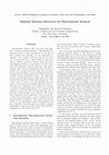The ranking results are also illustrated in Fig. 1 left and right, for the linear and kernel methods, respectively. The vertical axis in both figures depicts the various methods, while the horizontal axis depicts the performance ranking. The circles indicate the mean rank and the intervals around them indicate the confidence interval as this is determined by the CD value. Overlapping intervals between two methods indicate that there is not a statistically significant TABLE I: Cross Validation Classification Accuracies (%) of Linear Methods on Several Real-World Datasets DATASET FER-AIIA BU JAFFE KANADE MNIST SEMEION XM2VTS IONOSPHERE MONK 1 MONK 2 MONK 3 PIMA SPECIFIC RANK OVERALL RANK LPP PCA LDA MFA CDA SDA SMFA 40.9(3) 39.4(298) 46.8(18) 34.2(92) 71.1(259) 53.6(99) 95.7(54) 84.6(23) 66.7(3) 56.0(1) 77.2(5) 61.8(1) 31.0(120) 38.1(49) 37.6(39) 43.3(46) 79.9(135) 83.2(55) 92.0(86) 72.3(15) 68.3(5) 53.3(4) 80.9(4) 63.5(6) 64.6(6) 51.6(6) 53.2(6) 67.1(6) 84.6(9) 88.2(9) 70.5(1) 78.9(1) 50.8(1) 52.0(1) 49.4(1) 56.5(1) 72.6(10) 52.4(6) 61.5(14) 66.3(19) 82.8(38) 86.9(8) 97.7(4) 76.0(12) 71.7(2) 58.7(2) 81.6(1) 74.4(1) 73.2 49.1(16) 40.0(15) 59.7(7) 84.8(15) 89.2(19) 98.1(3) 80.6(2) 70.0(4) 54.2(1) 74.6(2) 60.5(3) 75.5(11) 52.3(15) 54.1(6) 67.1(5) 85.1(14) 89.4(19) 97.4(2) 83.4(2) 74.2(3) 54.0(2) 66.3(2) 73.5(3) 72.6(12) 49.3(11) 44.9(20) 63.8(9) 85.3(40) 87.5(10) 98.4(4) 84.3(26) 78.3(2) 60.7(1) 86.1(5) 74.9(1) 5.1 9.0 5.8 9.8 5.0 8.5 3.0 5.0 4.0 6.6 2.7 5.0 2.3 4.0 TABLE II: Cross Validation Classification Accuracies (%) of Kernel Methods on Several Real-World Datasets DATASET FER-AIIA BU JAFFE KANADE MNIST SEMEION XM2VTS IONOSPHERE MONK 1 MONK 2 MONK 3 PIMA SPECIFIC RANK OVERALL RANK KLPP KPCA KDA KMFA KCDA KSDA KSMFA 50.2(252) 52.7(317) 28.8(98) 32.7(99) 81.4(299) 83.8(99) 71.3(297) 83.7(23) 63.3(2) 54.8(1) 62.5(2) 50.7(3) 41.5(29) 35.9(290) 25.9(58) 33.2(88) 64.5(155) 77.4(77) 74.7(56) 70.3(2) 72.5(1) 59.8(3) 79.2(5) 67.5(4) 54.9(6) 46.6(6) 42.4(6) 44.3(6) 86.0(9) 95.3(9) 61.3(1) 92.9(1) 55.8(1) 69.7(1) 51.7(1) 48.9(1) 61.3(9) 44.4(29) 47.8(6) 46.6(6) 86.4(21) 90.0(11) 78.7(31) 92.3(1) 60.0(1) 70.8(2) 79.2(2) 54.0(3) 56.1(12) 41.0(13) 36.1(18) 40.0(6) 83.4(19) 94.1(19) 71.5(3) 93.1(1) 58.3(4) 78.7(1) 67.5(2) 52.5(3) 53.5(12) 48.0(14) 46.3(5) 38.5(6) 85.2(15) 95.9(19) 57.3(4) 92.9(1) 61.7(3) 54.5(1) 58.3(1) 52.9(1) 56.7(39) 39.9(18) 34.1(13) 45.8(7) 86.7(34) 94.9(20) 81.2(4) 92.6(1) 70.8(4) 79.7(2) 73.3(2) 56.2(3) 5.3 10.2 5.0 10.0 4.3 8.1 2.8 6.3 3.9 8.2 4.1 8.3 2.6 6.1 difference between the corresponding ranks. The first remark from Tables I,II and Fig. 1 is that SMFA and KSMFA outperform the rest methods in the linear and kernel case, respectively. Although their superiority is not statistically significant over all remaining methods, undoubtedly these two methods offer a strong potential to improve the performance or the state-of-the-art in many classification domains. In addition, it is interesting to observe the robustness of SMFA and MFA along with their kernel counterparts across the datasets. This observation combined with the fact that both these methods rely on the same motivations shows the advantage gained by encoding the data distributions using neighbouring information between the samples towards overcoming the several limitations previously presented in this paper, offering at the same time great generalization chances. As a general remark, the superiority of subclass methods against unimodal ones is evident, with MFA and KMFA being vivid exceptions. The top overall performance is shown by SMFA followed by SDA and MFA, while the worst performance is shown by KLPP. More specifically, on the one hand, SDA, MFA and KMFA display on average the best performance in facial expression recognition problems. On the other hand, in optical digit recognition, face frontal view recognition and the remaining classification problems, SMFA and KSMFA clearly have on average the optimal performance. In comparing linear with kernel methods, a simple calculation yields mean overall rank equal to 6.84 for the linear methods and 8.17 for the kernel ones. Although the difference between the two approaches (i.e., linear and kernel) is significant, we must admit that there is ample space for improving the kernel results by varying the RBF parameter, as the selection of this parameter is not trivial and may easily lead to over-fitting. Actually, the top performance rates presented in this paper have been obtained by testing indicative values of the above parameter. As a matter of fact, it is interesting to observe that the use of kernels proves to be beneficial for some LPP KLPP PCA KPCA LDA KDA MFA KMFA CDA KCDA SDA KSDA SMFA KSMFA 1 2 3 4 5 6 7 8 1 Rank 2 3 4 Rank 5 6 7 Fig. 1: Ranking of Various Methods After Pairwise Post-Hoc Bonferroni Tests on Real Data. (Left: Linear Methods, Right: Kernel Methods) methods in certain datasets, while deteriorates the performance of others. For instance, from Tables I and II, the use of kernels boosts the performance of PCA in three out of the four last datasets (i.e., MONK 1, MONK 3 and PIMA), while this is not the case for example in XM2VTS. There are two main reasons for this. Firstly, while some datasets contain linearly separable classes, others may need some kernel to obtain this linearity. The second reason is that in our experiments, for relaxing the computational complexity, we have used the same kernel values per dataset across all methods and there is no fact advocating that the same value constitutes the optimal parameter for each method. VI. C ONCLUSIONS The main contribution of this paper is a novel Subclass Marginal Fisher Analysis (SMFA) dimensionality reduction method. The functionality of SMFA is based on adjacency information of data samples within the same subclass as well as the proximity of “marginal” samples belonging to different classes. In this way, the new method combines the flexibility of neighbourhood modelling methods, like MFA, with the modularity offered by subclass information towards overcoming inherent limitations stemming from the data distributions, offering at the same moment great generalization chances. Through an extensive experimental study, it has been shown that SMFA outperforms a number of state-of-the-art subspace learning methods in many real-world datasets pertaining to various classification domains. Similar remarks could also be drawn for KSMFA. Moreover, as a general remark, it could be stated that subclass-based methods exhibit supe- rior performance against unimodal ones, in terms of classification accuracy, proving the potential of including subclass information in the dimensionality reduction process. Although the performance of the proposed method is impressive, there is yet space for exploring new methods employing the Graph Embedding framework, either by designing completely new methods or by modifying SMFA. Experimenting on this direction is encompassed in our future plans. Moreover, in order to reinforce even more the outcomes of this paper and to provide more credibility to SMFA, in the near future we intend to extend our current experimental study to more datasets from additional classification domains. R EFERENCES [1] [2] [3] [4] [5] [6] [7] X. He and P. Niyogi, “Locality preserving projections,” in NIPS, S. Thrun, L. K. Saul, and B. Schölkopf, Eds. MIT Press, 2003. X. He, S. Yan, Y. Hu, P. Niyogi, and H. Zhang, “Face recognition using laplacianfaces,” IEEE Trans. Pattern Anal. Mach. Intell, vol. 27, no. 3, pp. 328–340, 2005. I. Jolliffe, Principal Component Analysis. Springer Verlag, 1986. D. J. Kriegman, J. P. Hespanha, and P. N. Belhumeur, “Eigenfaces vs. fisherfaces: Recognition using classspecific linear projection,” in ECCV, 1996, pp. I:43–58. X. W. Chen and T. S. Huang, “Facial expression recognition: A clustering-based approach,” Pattern Recognition Letters, vol. 24, no. 9-10, pp. 1295–1302, Jun. 2003. M. L. Zhu and A. M. Martinez, “Subclass discriminant analysis,” IEEE Trans. Pattern Analysis and Machine Intelligence, vol. 28, no. 8, pp. 1274–1286, Aug. 2006. S. Yan, D. Xu, B. Zhang, H.-J. Zhang, Q. Yang, and S. Lin, “Graph embedding and extensions: A general framework for dimensionality reduction,” Pattern Analysis and Machine Intelligence, IEEE Transactions on, vol. 29, no. 1, pp. 40–51, 2007. [8] J. Ye, R. Janardan, C. H. Park, and H. Park, “An optimization criterion for generalized discriminant analysis on undersampled problems.” IEEE Transactions on Pattern Analysis and Machine Intelligence (PAMI), vol. 26, no. 8, pp. 982–994, 2004. [25] [26] [9] M. Zhu and A. M. Martı́nez, “Pruning noisy bases in discriminant analysis,” IEEE Transactions on Neural Networks, vol. 19, no. 1, pp. 148–157, 2008. [27] [10] W. J. Krzanowski, P. Jonathan, W. V. McCarthy, and M. R. Thomas, “General interest section: Discriminant analysis with singular covariance matrices: Methods and applications to spectroscopic data.” Applied Statistics, vol. 44, no. 1, pp. 101–115, 1995. [28] [11] J. H. Friedman, “Regularized discriminant analysis,” Journal of the American Statistical Association, vol. 84, no. 405, pp. 165–175, 1989. [30] [12] M. Kyperountas, A. Tefas, and I. Pitas, “Weighted piecewise lda for solving the small sample size problem in face verification,” IEEE Transactions on Neural Networks, vol. 18, no. 2, pp. 506–519, 2007. [13] O. C. Hamsici and A. M. Martinez, “Bayes optimality in linear discriminant analysis,” IEEE Trans. Pattern Analysis and Machine Intelligence, vol. 30, no. 4, pp. 647–657, Apr. 2008. [29] [31] [32] [14] T. Hastie, A. Buja, and R. Tibshirani, “Penalized discriminant analysis,” Annals of Statistics, vol. 23, pp. 73–102, 1995. [33] [15] G. Baudat and F. Anouar, “Generalized discriminant analysis using a kernel approach,” Neural Computation, vol. 12, no. 10, pp. 2385–2404, 2000. [34] [16] M. Loog, R. P. W. Duin, and R. Haeb-Umbach, “Multiclass linear dimension reduction by weighted pairwise fisher criteria.” IEEE Transactions on Pattern Analysis and Machine Intelligence (PAMI), vol. 23, no. 7, pp. 762–766, 2001. [17] G. Goudelis, S. Zafeiriou, A. Tefas, and I. Pitas, “Classspecific kernel-discriminant analysis for face verification,” IEEE Transactions on Information Forensics and Security, vol. 2, no. 3-2, pp. 570–587, 2007. [18] N. Gkalelis, V. Mezaris, and I. Kompatsiaris, “Mixture subclass discriminant analysis,” Signal Processing Letters, IEEE, vol. 18, no. 5, pp. 319–322, 2011. [19] S. K. Zhou and R. Chellappa, “Multiple-exemplar discriminant analysis for face recognition.” International Conference on Pattern Recognition (ICPR) (4), pp. 191–194, 2004. [20] X. Wu, X. Chen, X. Li, L. Zhou, and J. Lai, “Adaptive subspace learning: an iterative approach for document clustering,” Neural Computing and Applications, pp. 1–10. [21] X. Shu, Y. Gao, and H. Lu, “Efficient linear discriminant analysis with locality preserving for face recognition,” Pattern Recognition, vol. 45, no. 5, pp. 1892–1898, 2012. [22] K.-R. Müller, S. Mika, G. Rätsch, S. Tsuda, and B. Schölkopf, “An introduction to kernel-based learning algorithms.” IEEE Transactions on Neural Networks, vol. 12, no. 2, pp. 181–202, 2001. [23] B. Schölkopf, A. J. Smola, and K.-R. Muller, “Kernel principal component analysis.” in Proceedings of the International Conference on Artificial Neural Networks (ICANN1997), 1997, pp. 583–588. [24] M.-H. Yang, “Kernel eigenfaces vs. kernel fisherfaces: [35] Face recognition using kernel methods.” in FGR. IEEE Computer Society, 2002, pp. 215–220. B. Ma, H. Y. Qu, and H. S. Wong, “Kernel clustering-based discriminant analysis,” Pattern Recognition, vol. 40, no. 1, pp. 324–327, Jan. 2007. D. You, O. C. Hamsici, and A. M. Martı́nez, “Kernel optimization in discriminant analysis,” IEEE Trans. Pattern Anal. Mach. Intell., vol. 33, no. 3, pp. 631–638, 2011. G. J. McLachlan and T. Krishnan, The EM algorithm and extensions., 2nd ed., ser. Wiley series in probability and statistics. Hoboken, NJ: Wiley, 2008. Doob, “Spectral graph theory.” in Handbook of Graph Theory, CRC Press, 2004, J. L. Gross and J. Yellen, Eds., 2004. U. von Luxburg, “A tutorial on spectral clustering,” Statistics and Computing, vol. 17, no. 4, pp. 395–416, 2007. U. von Luxburg, O. Bousquet, and M. Belkin, “Limits of spectral clustering.” in Advances in Neural Information Processing Systems (NIPS), vol. 17. MIT Press, 2005, pp. 857–864. A. Azran and Z. Ghahramani, “Spectral methods for automatic multiscale data clustering.” in IEEE Computer Vision and Pattern Recognition (CVPR) (1). IEEE Computer Society, 2006, pp. 190–197. A. Maronidis, A. Tefas, and I. Pitas, “Frontal view recognition using spectral clustering and subspace learning methods.” in ICANN (1), ser. Lecture Notes in Computer Science, W. D. K. I. Diamantaras and L. S. Iliadis, Eds., vol. 6352. Springer, 2010, pp. 460–469. O. J. Dunn, “Multiple comparisons among means,” Journal of American Statistical Association, vol. 56, no. 293, pp. 52–64, 1961. H. Chen, P. Tino, and X. Yao, “Probabilistic classification vector machines.” IEEE Transactions on Neural Networks, vol. 20, no. 6, pp. 901–914, 2009. J. Demsar, “Statistical comparisons of classifiers over multiple data sets,” Journal of Machine Learning Research, vol. 7, pp. 1–30, 2006.