EURASIP Journal on Applied Signal Processing 2002:11, 1248–1259 c 2002 Hindawi Publishing Corporation
A Support Vector Machine-Based Dynamic Network for Visual Speech Recognition Applications Mihaela Gordan Department of Informatics, Aristotle University of Thessaloniki, Box 451, Thessaloniki 54006, Greece Email: mihag@zeus.csd.auth.gr Constantine Kotropoulos Department of Informatics, Aristotle University of Thessaloniki, Box 451, Thessaloniki 54006, Greece Email: costas@zeus.csd.auth.gr Ioannis Pitas Department of Informatics, Aristotle University of Thessaloniki, Box 451, Thessaloniki 54006, Greece Email: pitas@zeus.csd.auth.gr Received 26 November 2001 and in revised form 26 July 2002 Visual speech recognition is an emerging research field. In this paper, we examine the suitability of support vector machines for visual speech recognition. Each word is modeled as a temporal sequence of visemes corresponding to the different phones realized. One support vector machine is trained to recognize each viseme and its output is converted to a posterior probability through a sigmoidal mapping. To model the temporal character of speech, the support vector machines are integrated as nodes into a Viterbi lattice. We test the performance of the proposed approach on a small visual speech recognition task, namely the recognition of the first four digits in English. The word recognition rate obtained is at the level of the previous best reported rates. Keywords and phrases: visual speech recognition, mouth shape recognition, visemes, phonemes, support vector machines, Viterbi lattice. 1. INTRODUCTION Audio-visual speech recognition is an emerging research field where multimodal signal processing is required. The motivation for using the visual information in performing speech recognition lays on the fact that the human speech production is bimodal by its nature. In particular, human speech is produced by the vibration of the vocal cords and depends on the configuration of the articulatory organs, such as the nasal cavity, the tongue, the teeth, the velum, and the lips. A speaker produces speech using these articulatory organs together with the muscles that generate facial expressions. Because some of the articulators, such as the tongue, the teeth, and the lips are visible, there is an inherent relationship between the acoustic and visible speech. As a consequence, the speech can be partially recognized from the information of the visible articulators involved in its production and in particular from the image region comprising the mouth [1, 2, 3]. Undoubtedly, the most useful information for speech recognition is carried by the acoustic signal. When the acoustic speech is clean, performing visual speech recognition and integrating the recognition results from both modalities does not bring too much improvement because the recognition rate from the acoustic information alone is very high, if not perfect. However, when the acoustic speech is degraded by noise, adding the visual information to the acoustic one improves significantly the recognition rate. Under noisy conditions, it has been proved that the use of both modalities for speech recognition is equivalent to a gain of 12 dB in the signal-to-noise ratio of the acoustic signal [1]. For large vocabulary speech recognition tasks, the visual signal can also provide a performance gain when it is integrated with the acoustic signal, even in the case of a clean acoustic speech [4]. Visual speech recognition refers to the task of recognizing the spoken words based only on the visual examination of the speaker’s face. This task is also referred to as lipreading, since the most important visible part of the face examined for information extraction during speech is the mouth area. Different shapes of the mouth (i.e., different mouth openings and different position of the teeth and tongue) realized during speech cause the production of different sounds. We can establish a correspondence between the mouth shape and A Support Vector Machine-Based Dynamic Network for Visual Speech Recognition Applications the phone produced, even if this correspondence is not oneto-one, but one-to-many, due to the involvement of invisible articulatory organs in the speech production. For small vocabulary word recognition tasks, we can perform good quality speech recognition using the visual information conveyed by the mouth shape only. Several methods have been reported in the literature for visual speech recognition. The adopted methods vary widely with respect to: (1) the feature types, (2) the classifier used, and (3) the class definition. For example, Bregler and Omohundro [5] used time delayed neural networks (TDNN) for visual classification and the outer lip contour coordinates as visual features. Luettin and Thacker [6] used active shape models to represent the different mouth shapes and gray level distribution profiles (GLDPs) around the outer and/or inner lip contours as feature vectors, and finally built whole-word hidden Markov model (HMM) classifiers for visual speech recognition. Movellan [7] employed also HMMs to build the visual word models, but he used directly the gray levels of the mouth images as features after simple preprocessing to exploit the vertical symmetry of the mouth. In recent works, Movellan et al. [8] have reported very good results when partially observable stochastic differential equation (SDE) models are integrated in a network as visual speech classifiers instead of HMMs, and Gray et al. [9] have presented a comparative study of a series of different features based on principal component analysis (PCA) and independent component analysis (ICA) in an HMM-based visual speech recognizer. Despite the variety of existing strategies for visual speech recognition, there is still ongoing research in this area attempting to: (1) find the most suitable features and classification techniques to discriminate effectively between the different mouth shapes, while preserving in the same class the mouth shapes produced by different individuals that correspond to one phone; (2) require minimal processing of the mouth image to allow for a real time implementation of the mouth shape classifier; (3) facilitate the easy integration of audio and video speech recognition modules [1]. In this paper, we contribute to the first two of the aforementioned aspects in visual speech recognition by examining the suitability of support vector machines (SVMs) for visual speech recognition tasks. The idea is based on the fact that SVMs have been proved powerful classifiers in various pattern recognition applications, such as face detection, face verification/recognition, and so forth [10, 11, 12, 13, 14, 15]. Very good results in audio speech recognition using SVMs were recently reported in [16]. No attempts in applying SVMs for visual speech recognition have been reported so far. According to the authors’ knowledge, the use of SVMs as visual speech classifiers is a novel idea. One of the reasons that partially explains why SVMs have not been exploited in automatic speech recognition so far is that they are inherently static classifiers, while speech is a dynamic process where the temporal information is essential for recognition. A solution to this problem was presented in [16] where a combination of HMMs with SVMs is proposed. In this paper, a similar strategy is adopted. We will use Viterbi lattices to create dynamically visual word models. 1249 The approaches for building the word models can be classified into the approaches where whole word models are developed [6, 7, 16] and those where viseme-oriented word models are derived [17, 18, 19]. In this paper, we adopt the latter approach because it is more suitable for an SVM implementation and offers the advantage of an easy generalization to large vocabulary word recognition tasks without a significant increase in storage requirements. It maintains also the dictionary of basic visual models needed for word modeling into a reasonable limit. The word recognition rate obtained is on the level of the best previous reported rates in literature, although we will not attempt to learn the state transition probabilities. When very simple features (i.e., pixels) are used, our word recognition rate is superior to the ones reported in the literature. Accordingly, SVMs are a promising alternative for visual speech recognition and this observation encourages further research in that direction. It is well known that the MortonMassaro law (MML) holds when humans integrate audio and visual speech [20]. Experiments have demonstrated that MML holds also for audio-visual speech recognition systems. That is, the audio and visual speech signals may be treated as if they were conditionally independent without significant loss of information about speech categories [20]. This observation supports the independent treatment of audio and visual speech and yields an easy integration of the visual speech recognition module and the acoustic speech recognition module. The paper is organized as follows. In Section 2, a short overview on SVM classifiers is presented. We review the concepts of visemes and phonemes in Section 3. We discuss the proposed SVM-based approach to visual speech recognition in Section 4. Experimental results obtained when the proposed system is applied to a small vocabulary visual speech recognition task (i.e., the visual recognition of the first four digits in English) are described in Section 5 and compared to other results published in the literature. Finally, in Section 6, our conclusions are drawn and future research directions are identified. 2. OVERVIEW ON SVMS AND THEIR APPLICATIONS IN PATTERN RECOGNITION SVMs constitute a principled technique to train classifiers that stems from statistical learning theory [21, 22]. Their root is the optimal hyperplane algorithm. They minimize a bound on the empirical error and the complexity of the classifier at the same time. Accordingly, they are capable of learning in sparse high-dimensional spaces with relatively few training examples. Let {xi , yi }, i = 1, 2, . . . , N, denote N training examples where xi comprises an M-dimensional pattern and yi is its class label. Without loss of generality, we will confine ourselves to the two-class pattern recognition problem. That is, yi ∈ {−1, +1}. We agree that yi = +1 is assigned to positive examples, whereas yi = −1 is assigned to counterexamples. The data to be classified by the SVM might or might not be linearly separable in their original domain. If they are 1250 EURASIP Journal on Applied Signal Processing separable, then a simple linear SVM can be used for their classification. However, the power of SVMs is demonstrated better in the nonseparable case when the data cannot be separated by a hyperplane in their original domain. In the latter case, we can project the data into a higher-dimensional Hilbert space and attempt to linearly separate them in the higher-dimensional space using kernel functions. Let Φ denote a nonlinear map Φ : RM → Ᏼ where Ᏼ is a higherdimensional Hilbert space. SVMs construct the optimal separating hyperplane in Ᏼ. Therefore, their decision boundary is of the form f (x) = sign
N     αi yi K x, xi + b , i=1 (1) where K(z1 , z2 ) is a kernel function that defines the dot product between Φ(z1 ) and Φ(z2 ) in Ᏼ, and αi are the nonnegative Lagrange multipliers associated with the quadratic optimization problem that aims to maximize the distance between the two classes measured in Ᏼ subject to the constraints wT Φ xi + b ≥ 1 T     w Φ xi + b ≤ 1 for yi = +1, for yi = −1, (2) where w and b are the parameters of the optimal separating hyperplane in Ᏼ. That is, w is the normal vector to the hyperplane, |b|/ w is the perpendicular distance from the hyperplane to the origin, and w denotes the Euclidian norm of vector w. The use of kernel functions eliminates the need for an explicit definition of the nonlinear mapping Φ, because the data appears in the training algorithm of SVM only as dot products of their mappings. Frequently used, kernel functions are the polynomial kernel K(xi , x j ) = (mxiT x j + n)q and the radial basis function (RBF) kernel K(xi , x j ) = exp{−γ|xi − x j |2 }. In the following, we omit the sign function from the decision boundary (1) that simply makes the optimal separating hyperplane an indicator function. To enable the use of SVM classifiers in visual speech recognition when we model the speech as a temporal sequence of symbols corresponding to the different phones produced, we will employ the SVMs as nodes in a Viterbi lattice. But the nodes of such a Viterbi lattice should generate the posterior probabilities for the corresponding symbols to be emitted [23] and the standard SVMs do not provide such probabilities as output. Several solutions are proposed in the literature to map the SVM output to probabilities: the cosine decomposition proposed by Vapnik [21], the probabilistic approximation by applying the evidence framework to SVMs [24], and the sigmoidal approximation by Platt [25]. Here we adopt the solution proposed by Platt [25] since it is a simple solution which was already used in a similar application of SVMs to audio speech recognition [16]. The solution proposed by Platt shows that having a trained SVM, we can convert its output to probability by training the parameters a1 and a2 of a sigmoidal mapping function, and that this produces a good mapping from SVM margins to probability. In general, the class-conditional densities on either side of the SVM hyperplane are exponential. So, Bayes’ rule [26] on two exponentials suggests the use of the following parametric form of a sigmoidal function:   P y = +1 | f (x) = where 1  , 1 + exp a1 f (x) + a2 (3) (i) y is the label for x, given by the sign of f (x) (y = +1 if and only if f (x) > 0), (ii) f (x) is the function value on the output of an SVM classifier for the feature vector x to be classified, (iii) a1 and a2 are the parameters of the sigmoidal mapping to be derived for the currently trained SVM under consideration with a1 < 0. P(y = −1 | f (x)) could be defined similarly. However, since each SVM represents only one data category (i.e., the positive examples), we are interested only in the probability given by (3). The latter equation gives directly the posterior probability to be used in a Viterbi lattice. The parameters a1 and a2 are derived from a training set ( f (xi ), yi ) using maximum likelihood estimation. In the adopted approach, we use the training set of the SVM, (xi , yi ), i = 1, 2, . . . , N, to estimate the parameters of the sigmoidal function. The estimation starts with the definition of a new training set, ( f (xi ), ti ), i = 1, 2, . . . , N, where ti are the target probabilities. The target probabilities are defined as follows. (i) When a positive example (i.e., yi = +1) is observed at a value f (xi ), we assume that this example is probably in the class represented by the SVM, but there is still a small finite probability ǫ+ for getting the opposite label at the same f (xi ) for some out-of-sample data. Thus, ti = t+ = 1 − ǫ+. (ii) When a negative example (i.e., yi = −1) is observed at a value f (xi ), we assume that this example is probably not in the class represented by the SVM, but there is still a small finite probability ǫ− for getting the opposite label at the same f (xi ) for some out-of-sample data. Thus, ti = t− = ǫ−. Denote by N+ the number of positive examples in the training set (xi , yi ), i = 1, 2, . . . , N. Let N− be the number of negative examples in the training set. We set t+ = 1 − ǫ+ = (N+ + 1)/(N+ + 2) and t− = ǫ− = 1/(N− + 2). The parameters a1 and a2 are found by minimizing the negative log likelihood of the training data which is a crossentropy error function given by   Ᏹ a1 , a2 = − N  i=1       ti log pi + 1 − ti log 1 − pi , (4) where   t+ , ti =  pi = t− , for yi = +1, for yi = −1, 1    . 1 + exp a1 f xi + a2 (5) (6) A Support Vector Machine-Based Dynamic Network for Visual Speech Recognition Applications 1251 In (4) and (6), pi , i = 1, 2, . . . , N, is the value of the sigmoidal mapping for the training example xi , where f (xi ) is the realvalued output of the SVM for this example. Due to the negative sign of a1 , pi tends to 1 if xi is a positive example (i.e., f (xi ) > 0) and to 0 if xi is a negative example (i.e., f (xi ) < 0). 3. VISEMES AND PHONEMES 3.1. Phonetic word description The basic units of the acoustic speech are the phones. Roughly speaking, a phone is an acoustic realization of a phoneme, a theoretical unit for describing how speech conveys linguistic meaning. The acoustic realization of a phoneme depends on the speaker’s characteristics, the word context, and so forth. The variations in the pronunciation of the same phoneme are called allophones. In the technical literature, a clear distinction between phones and phonemes is seldom made. In this paper, we are dealing with speech recognition in English, so we will focus on this particular case. The number of phones in the English language varies in the literature [27, 28]. Usually there are about 10–15 vowels or vowellike phones and 20–25 consonants. The most commonly used computer-based phonetic alphabet in American English is ARPABET which consists of 48 phones [2]. To convert the orthographic transcription of a word in English to its phonetic transcription, we can use the publicly available Carnegie Mellon University (CMU) pronunciation dictionary [29]. The CMU pronunciation dictionary uses a subset of the ARPABET consisting of 39 phones. For example, the CMU phonetic transcription of the word “one” is “W-AHN”. 3.2. The concept of viseme Similarly to the acoustic domain, we can define the basic unit of speech in the visual domain, the viseme. In general, in the visual domain, we observe the image region of the speaker’s face that contains the mouth. Therefore, the concept of viseme is usually defined in relation to the mouth shape and the mouth movements. An example where the concept of viseme is related to the mouth dynamics is the viseme OW which represents the movement of the mouth from a position close to O to a position close to W [2]. In such a case, to represent a viseme, we need to use a video sequence, a fact that would complicate the processing of the visual speech to some extent. 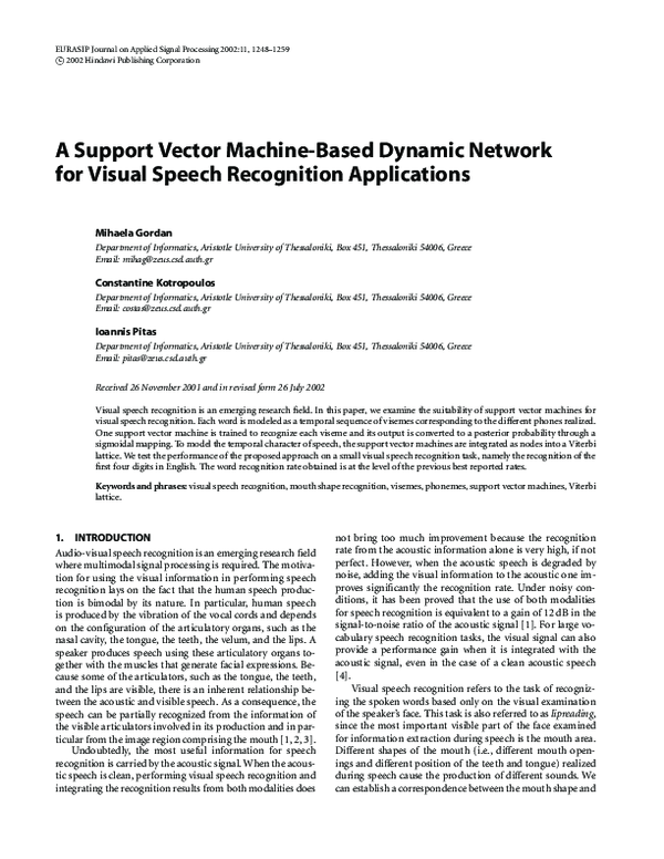However, fortunately, most of the visemes can be approximately represented by stationary mouth images. Two examples of visemes defined in relation to the mouth shape during the production of the corresponding phones are given in Figure 1. 3.3. Phoneme to viseme mappings To be able to perform visual speech recognition, ideally we would like to define for each phoneme its corresponding viseme. In this way, each word could be unambiguously described according to its pronunciation in the visual domain. Unfortunately, invisible articulatory organs are also involved in speech production that renders the mapping of phonemes (a) (b) Figure 1: (a) Mouth shape during the realization of phone /O/; (b) mouth shape during the realization of phone /F/, by the subject Anthony in the Tulips1 database [7]. Table 1: The most used viseme groupings for the English consonants [1]. Viseme group index Corresponding consonants 1 2 3 4 5 6 7 8 9 /F/; /V/ /TH/; /DH/ /S/; /Z/ /SH/; /ZH/ /P/; /B/; /M/ /W/ /R/ /G/; /K/; /N/; /T/; /D/; /Y/ /L/ to visemes into many-to-one. Thus, there are phonemes that cannot be distinguished in the visual domain. For example, the phonemes /P/, /B/, and /M/ are all produced with a closed mouth and are visually indistinguishable, so they will be represented by the same viseme. We also have to consider the dual aspect corresponding to the concept of allophones in the acoustic domain. The same viseme can have different realizations represented by different mouth shapes due to the speaker variability and the context. Unlike the phonemes, in the case of visemes there are no commonly accepted viseme tables by all researchers [1], although several attempts toward this direction have been undertaken. For example, it is commonly agreed that the visemes of the English consonants can be grouped into 9 distinct groups, as in Table 1 [1]. To obtain the viseme groupings, the confusions in stimulus-response matrices measured on an experimental basis are analyzed. In such experiments, subjects are asked to visually identify syllables in a given context such as vowel-consonant-vowel (V-C-V) words. Then, the stimulus-response matrices are tabulated and the visemes are identified as those clusters of phonemes in which at least 75% of all responses occur. This strategy will lead to a systematic and application-independent mapping of phonemes to visemes. Average linkage hierarchical clustering [18] and self-organizing maps [17] were employed to group visually similar phonemes based on geometric features. Similar techniques could be applied for raw images from mouth regions as well. 1252 However, in this paper, we do not resort to such strategies because our main goal is the evaluation of the proposed visual speech recognition method. Thus, we define only those visemes that are strictly needed to represent the visual realization of the small vocabulary used in our application and manually classify the training images to a number of predefined visemes, as explained in Section 5. 4. THE PROPOSED APPROACH TO VISUAL SPEECH RECOGNITION Depending on the approach used to model the spoken words in the visual domain, we can classify the existing visual speech recognition systems to systems using word-oriented models and those using viseme-oriented models [4]. In this paper, we develop viseme-oriented models. Visemic-based lipreading was investigated also in [17, 18]. Each visual word model can be represented afterwards as a temporal sequence of visemes. Thus, the structure of the visual word modeling and recognition system can be regarded as a two-level structure. (1) At the first level, we build the viseme classes, one class of mouth images for each viseme defined. This implies the formulation of the mouth shape recognition problem as a pattern recognition problem. The patterns to be recognized are the mouth shapes, symbolically represented as visemes. In our approach, the classification of mouth shapes to viseme classes is formulated as a two-class (binary) pattern recognition problem and there is one SVM dedicated for each viseme class. (2) At the second level, we build the abstract visual word models described as temporal sequences of visemes. The visual word models are implemented by means of the Viterbi lattices where each node generates the emission probability of a certain viseme at one particular time instant. Notice that the aforementioned two-level approach is very similar to some techniques employed for acoustic speech recognition [16], justifying thus our expectation that the proposed method will ensure an easy integration of the visual speech recognition subsystem with a similar acoustic speech recognition subsystem. In this section, we focus on the first level of the proposed algorithm for visual speech modeling and recognition. The second level involves the development of the visual symbolic sequential word models using the Viterbi lattices. The latter level is discussed only in principle. 4.1. Formulation of visual speech recognition as a pattern recognition problem The problem of discriminating between different mouth shapes during speech production can be viewed as a pattern recognition problem. In this case, the set of patterns is a set of feature vectors {xi }, i = 1, 2, . . . , P, each of them describing some mouth shape. The feature vector xi is a representation of the mouth image. The feature vector xi can represent the mouth image at low level (i.e., the gray levels from a rectangular image region containing the mouth). It can comprise geometric parameters (i.e., mouth width, height, EURASIP Journal on Applied Signal Processing perimeter, etc.) or the coefficients of a linear transformation of the mouth image. All the feature vectors from the set have the same number of components M. Denote the pattern classes by Ꮿ j , j = 1, 2, . . . , Q, where Q is the total number of classes. Each class Ꮿ j is a group of patterns that represent mouth shapes corresponding to one viseme. A network of Q parallel SVMs is designed where each SVM is trained to classify test patterns in class Ꮿ j or its complement ᏯCj . We should slightly deviate from the notation introduced in Section 2 because a test pattern xi could be assigned to more than one class. It is convenient to represent the class label of a test pattern, xk , by a (Q × 1) vector yk whose jth element, yk j , admits the value 1 if xk ∈ Ꮿ j and −1 otherwise. It may occur more than one element of yk to have the value 1 if f j (xk ) > 0, where f j (xk ) is the decision function of the jth SVM. To derive an unambiguous classification, we will use SVMs with probabilistic outputs, that is, the output of the jth SVM classifier will be the posterior probability for the test pattern xk to belong to the class Ꮿ j , P(y j = 1 | f j (xk )), given by (3). This pattern recognition problem can be applied to visual speech recognition in the following way: (i) each unknown pattern represents the image of the speaker’s face at a certain time instant; (ii) each class label represents one viseme. Accordingly, we will identify what the probability of a viseme to be produced at any time instant in the spoken sequence is. This gives the solution required at the first level of the proposed visual speech recognition system to be passed to the second level. The network of Q parallel SVMs is shown in Figure 2. 4.2. The basic structure of the SVM network for visual speech recognition The phonetic transcription represents each word by a left-toright sequence of phonemes. Moreover, the visemic model corresponding to the phonetic model of a word can be easily derived using a phoneme-to-viseme mapping. However, the aforementioned representation shows only which visemes are present in the pronunciation of the word, not the duration of each viseme. Let Ti , i = 1, 2, . . . , S, denote the duration of the ith viseme in a word model of S visemes. Let T be the duration of the video sequence that results from the pronunciation of this word. In order to align the video sequence of duration T with the symbolic visemic model of S visemes, we can create a temporal Viterbi lattice [23] containing as many states as the frames in the video sequence, that is, T. Such a Viterbi lattice that corresponds to the pronunciation of the word “one” is depicted in Figure 3. For this example, the visemes present in the word pronunciation have been denoted with the same symbols as the underlying phones. Let D be the total number of visemic models defined for the words in the vocabulary. Each visemic model wd , d = 1, 2, . . . , D, has its own Viterbi lattice. Each node in the A Support Vector Machine-Based Dynamic Network for Visual Speech Recognition Applications Visual features xk 1253 SVM1 p(y1 = 1 | f1 (xk )) SVM2 p(y2 = 1 | f2 (xk )) SVM3 p(y3 = 1 | f3 (xk )) . .. SVMQ p(yQ = 1 | fQ (xk )) Figure 2: Illustration of the parallel network of binary classifiers for viseme recognition. Visemic symbolic model The probability that the visemic word model wd is realized can be computed by ᏸ pd = max pℓ , N ℓ =1 AH W 1 2 3 4 5 Temporal frame Figure 3: A temporal Viterbi lattice for the pronunciation of the word “one” in a video sequence of 5 frames. lattice of Figure 3 is responsible for the generation of one observation that belongs to a certain class at each time instant. Let lk = 1, 2, . . . , Q be the class label where the observation ok generated at time instant k belongs to. Let us denote the emission probability of that observation by blk (ok ). Each solid line between any two nodes in the lattice represents a transition probability between two states. Denote by alk ,lk+1 the transition probability from the node corresponding to the class lk at time instant k to the node corresponding to the class lk+1 at time instant k + 1. The class labels lk and lk+1 may or may not be different. Having a video sequence of T frames for a word and a Viterbi lattice for each visemic word model wd , d = 1, 2, . . . , D, we can compute the probability that the visemic word model wd is realized, following a path ℓ in the Viterbi lattice as T −1 T pd,ℓ =   alk ,lk+1 . blk ok · k=1 k=1 (7) (8) where ᏸ is the number of all possible paths in the lattice. Among the words that can be realized following any possible path in any of the D Viterbi lattices, the word described by the model whose probability pd , d = 1, 2, . . . , D, is maximum (i.e., the most probable word) is finally recognized. In the visual speech recognition approach discussed in this paper, the emission probability blk (ok ) is given by the corresponding SVM, SV Mlk . To a first approximation, we assume equal transition probabilities alk ,lk+1 between any two states. Accordingly, it is sufficient to take into account only the probabilities blk (ok ), k = 1, 2, . . . , T, in the computation of the path probabilities pd,ℓ which yields the simplified equation T pd,ℓ =   blk ok . k =1 (9) Of course, learning the probabilities alk lk+1 from word models would yield a more refined modeling. This could be a topic of future work. 5. EXPERIMENTAL RESULTS To evaluate the recognition performance of the proposed SVM-based visual speech recognizer, we choose to solve the task of recognizing the first four digits in English. Towards this end, we used the small audiovisual database Tulips1 [7] frequently used in similar visual speech recognition experiments. While the number of the words is small, this database is challenging due to the differences in illumination conditions, ethnicity, and gender of the subjects. Also we must mention that, despite the small number of words 1254 EURASIP Journal on Applied Signal Processing Table 2: Viseme classes defined for the four words of the Tulips1 database [7]. Viseme group index Symbolic notation Viseme description 1 2 3 4 5 6 7 8 9 (W) (AO) (WAO) (AH) (N) (T) (TH) (IY) (F) Small-rounded open mouth state Larger-rounded open mouth state Medium-rounded open mouth state Medium ellipsoidal mouth state Medium open, not rounded, mouth state; teeth visible Medium open, not rounded, mouth state; teeth and tongue visible Medium open, not rounded Longitudinal open mouth state Almost closed mouth position; upper teeth visible, lower lip moved inside pronounced in the Tulips1 database compared to vocabularies for real-world applications, the portion of phonemes in English covered by these four words is large enough: 10 out of 48 appearing in the ARPABET table, that is, approximately 20%. Since we use viseme-oriented models and the visemes are actually just representations of phonemes in the visual domain, we can consider the results described in this section as significant. Solving the proposed task requires first the design of a particular visual speech recognizer according to the strategy presented in Section 4. The design involves the following steps: (1) (2) (3) (4) to define the viseme to phoneme mapping; to build the SVM network; to train the SVMs for viseme classification; to generate and implement the word models as Viterbi lattices. Then, we use the trained visual speech recognizer to assess its recognition performance in test video sequences. Table 3: Phoneme-to-viseme mapping used in the experiments conducted on the Tulips1 database [7]. Viseme group index Corresponding phonemes 1, 2, or 3 (depending on speaker’s pronunciation) /W/, /UW/, /AO/ 1 or 3 (depending on speaker’s pronunciation) /R/ 4 5 6 7 8 or 4 (depending on speaker’s pronunciation) /AH/ /N/ /T/ /TH/ 9 /F/ /IY/ 5.1. Experimental protocol We start the design of the visual speech recognizer with the definition of the viseme classes for the first four digits in English. We first obtain the phonetic transcriptions of the first four digits in English using the CMU pronunciation dictionary [29]: “one” → “W-AH-N” “two” → “T-UW” “three” → “TH-R-IY” “four” → “F-AO-R”. We then try to define the viseme classes so that (i) a viseme class includes as few phonemes as possible; (ii) we have as few different visual realizations of the same viseme as possible. The definition of viseme classes was based on the visual examination of the video part from the Tulips1 database. The clustering of the different mouth images into viseme classes was done manually on the base of the visual similarity of these images. By this procedure, we obtained the viseme classes described in Table 2 and the phoneme-to-viseme mapping given in Table 3. We have to define and train one SVM for each viseme. To employ SVMs, we should define the features to be used to represent each mouth image and select the kernel function to be used. Since the recognition and generalization performance of each SVM is strongly influenced by the selection of the kernel function and the kernel parameters, we devoted much attention to these issues. We trained each SVM using the linear, the polynomial, and the RBF as kernel functions. In the case of the polynomial kernel, the degree of the polynomial q was varied between 2 and 6. For each trained SVM, we compared the predicted error, precision, and recall on the training set, as computed by SVMLight [30], for the different kernels and kernel parameters. We finally selected the simplest kernel yielding the best values for these estimates. That kernel was the polynomial kernel of degree q = 3. The RBF kernel gave the same performance estimates with the polynomial kernel of degree q = 3 on the training set but at the A Support Vector Machine-Based Dynamic Network for Visual Speech Recognition Applications cost of a larger number of support vectors. A simple choice of a feature vector such as the collection of the gray levels from a rectangular region of fixed size containing the mouth, scanned row by row, is proved suitable whenever SVMs have been used for visual classification tasks [15]. More specifically, we used two types of features to conduct the visual speech recognition experiments. (i) The first type comprised the gray levels of a rectangular region of interest around the mouth, downsampled to the size 16 × 16. Each mouth image is represented by a feature vector of length 256. (ii) The second type represented each mouth image frame at the time T f by a vector of double size (i.e., 512) that comprised the gray levels of the rectangular region of interest around the mouth downsampled to the size 16 × 16, as previously. The temporal derivatives of the gray levels normalized to the range [0, Lmax − 1], where Lmax is the maximum gray level value in mouth image. The temporal derivatives are simply the pixel by pixel gray level differences between the frames T f and T f − 1. These differences are the so-called delta features. Some preprocessing of the mouth images was needed before training and testing the visual speech recognition system. It concerns the normalization of the mouth in scale, rotation, and position inside the image. Such a preprocessing is needed due to the fact that the mouth has different scale, position in the image, and orientation toward the horizontal axis from utterance to utterance depending on the subject and on its position in front of the camera. To compensate for these variations, we applied the normalization procedure of mouth images with respect to scale, translation, and rotation described in [6]. The visual speech recognizer was tested for speakerindependent recognition using the leave-one-out testing strategy for the 12 subjects in the Tulips1 database. This implies training the visual speech recognizer 12 times, each time using only 11 subjects for training and leaving the 12th out for testing. In each case, we trained first the SVMs, and then the sigmoidal mappings for converting the SVMs output to probabilities. The training set, for each SVM in each system configuration is defined manually. Only the video sequences, from the so-called Set 1 from the Tulips1 database, were used for training. The labeling of all the frames from Set 1 (a total of 48 video sequences) was done manually by visual examination of each frame. We examined the video only to label all the frames according to Table 3 except the transition frames between two visemes denoting differently the same viseme class for each subject. Finally, we compared the similarity of the frames corresponding to the same viseme and different subjects and decided if the classes could be merged. The disadvantage of this approach is the large time needed for labeling, which would not be needed if HMMs were used for segmentation. A compromise solution for labeling could be the use of an automatic solution for phoneme-level segmentation of the audio sequence and the use of this segmentation on the aligned video sequence also. Once the labeling was done, only the unambiguous positive and negative viseme examples were included in the train- 1255 ing sets. The feature vectors used in the training sets of all SVMs were the same. Only their labeling as positive or negative examples differs from one SVM to another. This leads to an unbalanced training set in the sense that the negative examples are frequently more than the positive ones. The configuration of the Viterbi lattice depends on the length of the test sequence through the number of frames Ttest of the sequence (as illustrated in Figure 3). It was generated automatically at runtime for each test sequence. The number of Viterbi lattices can be determined in advance, because it is equal to the total number of visemic word models. Thus, taking into account the phonetic descriptions for the four words of the vocabulary and the phoneme-to-viseme mappings in Table 3, we have 3 visemic word models for the word “one,” 3 models for “two,” 4 models for “three,” and 6 models for “four.” The multiple visemic models per word are due to the variability in speakers’ pronunciation. In each of the 12 leave-one-out tests, we have as test sequences, the video sequences corresponding to the pronunciation of the four words and there are two pronunciations available for each word and the speaker. This leads to a subtotal of 8 test sequences per system configuration, and a total of 12 × 8 = 96 test sequences for the visual speech recognizer. The complete visual speech recognizer was implemented in C++. We used the publicly available SVMLight toolkit modules for the training of the SVMs [30]. We implemented in C++, the module for learning the sigmoidal mappings of the SVMs output to probabilities and the module for generating the Viterbi lattice models based on SVMs with probabilistic outputs. All these modules were integrated into the visual speech recognition system whose architecture is structured into two modules: the training module and the test module. Two visual speech recognizers were implemented, trained, and tested with the aforementioned strategy. They differ in the type of features used. The first system (without delta features) did not include temporal derivatives in the feature vector, while the second (with delta features) included also temporal derivatives between two frames in the feature vector. 5.2. Performance evaluation In this section, we present the experimental results obtained with the proposed system with or without using delta features. Moreover, we compare these results to others reported in the literature for the same experiment on the Tulips1 database. The word recognition rates (WRR) have been averaged over the 96 tests obtained by applying the leave-one-out principle. Five figures of merit are provided. (1) The WRR per subject, obtained by the proposed method when delta features are used, is measured and compared to that by Luettin and Thacker [6] (Table 4). (2) The overall WRR for all subjects and pronunciations, with and without delta features, is reported compared to that obtained by Luettin and Thacker [6], Movellan [7], Gray et al. [9], and Movellan et al. [8] (Table 5). (3) The confusion matrix between the words actually 1256 EURASIP Journal on Applied Signal Processing Table 4: WRR for each subject in Tulips1 using: (a) SVM dynamic network with delta features; (b) active appearance model (AAM) for inner and outer lip contours and HMM with delta features [6]. Subject 1 Accuracy [%] (SVM-based dynamic network) 100 Accuracy [%] (AAM&HMM [6]) 2 75 3 4 5 6 7 8 9 10 11 12 100 100 87.5 100 87.5 100 100 62.5 87.5 87.5 100 87.5 87.5 75 100 100 75 100 100 75 100 87.5 Table 5: The overall WRR of the SVM dynamic network compared to that of other techniques. Method SVM-based dynamic network without delta features SVM-based dynamic network with delta features AAM and HMM shape + intensity inner + outer lip contour without delta features [6] AAM and HMM shape + intensity inner + outer lip contour with delta features [6] HMMs [7] without delta features HMMs [7] with delta features WRR [%] 76 90.6 87.5 90.6 60 89.93 blocked filter bank PCA/ICA (local) [9] unblocked filter bank PCA/ICA (local) [9] Diffusion network shape + intensity [8] 85.4 91.7 91.7 Method WRR [%] Global PCA and HMMs [9] 79.2 Global ICA and HMMs [9] 74 presented to the classifier and the words recognized is shown in Table 6 and compared to the average human confusion matrix [7] (Table 7) in percentages. (4) The accuracy of the viseme segmentations resulting from the Viterbi lattices. (5) The 95% confidence intervals for the WRRs of the several systems included in the comparisons (Table 8) that provide an estimate of the performance of the systems for a much larger number of subjects. We would like to note that human subjects untrained in lipreading achieved, under similar experimental conditions, a WRR of 89.93%, whereas the hearing impaired had an average performance of 95.49% [7]. From the examination of Table 5, it can be seen that our WRR is equal to the best rate reported in [6] and just 1.1% below the recently reported rates in [8, 9]. However, the features used in the proposed method are simpler than those used with HMMs to obtain the same or higher WRRs. For the shape + intensity models [6], the gray levels should be sampled in the exact subregion of the mouth image containing the lips and around the inner and outer lip contours. It should also exclude the skin areas. Accordingly, the method reported in [6] requires the tracking of the lip contour in each frame which increases the processing time of visual speech recognition. For the method reported in [9], a large amount of local processing is needed, by the use of a bank of linear shift invariant filters with unblocked selection whose response filters are ICA or PCA kernels of very small size (12 × 12 pixels). The obtained WRR is higher than those reported in [7] where similar features are used, namely the gray levels of the region of interest (ROI) comprising the mouth after some simple preprocessing steps. The preprocessing in [7] was vertical symmetry enforcement of the mouth image by averaging, followed by low pass filtering, subsampling, and thresholding. Another measure of the performance assessment is given Table 6: Confusion matrix for visual word recognition by the dynamic network of SVMs with delta features. Digit recognized One Two Three Four One 95.83% 0.00% 0.00% 4.17% Digit presented Two 0.00% 95.83% 4.17% 0.00% Three 16.66% 12.5% 70.83% 0.00% Four 0.00% 0.00% 0.00% 100% Table 7: Average human confusion matrix [7]. Digit recognized One Two Three Four One 89.36% 0.46% 8.33% 1.85% Digit presented Two 1.39% 98.61% 0.00% 0.00% Three 9.25% 3.24% 85.64% 1.87% Four 4.17% 0.46% 1.85% 93.52% by comparing the confusion matrix of the proposed system with the average human confusion matrix provided in [7]. The accuracy of the viseme segmentation that results from the best Viterbi lattices was computed using, as reference, the manually performed segmentation of frames into the viseme classes (Table 3) as a percentage of the correctly classified frames. We obtained an accuracy of 89.33%, which is just 1.27% lower than the WRR. The results obtained demonstrate that the SVM-based dynamic network is a very promising alternative to the existing methods for visual speech recognition. An improvement of the WRR is expected, when the training of the transition A Support Vector Machine-Based Dynamic Network for Visual Speech Recognition Applications 1257 Table 8: 95% confidence interval for the WRR of the proposed system compared to that of other techniques. Method SVM-based dynamic network without delta features SVM-based dynamic network with delta features AAM and HMM shape + intensity inner + outer lip contour without delta features [6] Confidence interval [%] [66.6,83.5] [83.1,94.7] [79.4,92.7] [83.1,94.7] Global PCA & HMMs [9] Global ICA & HMMs [9] blocked filter bank PCA/ICA (local) [9] unblocked filter bank PCA/ICA (local) [9] Diffusion network shape + intensity [8] [70.0,86.1] [64.4,81.7] [76.9,91.1] [84.4,95.7] [84.4,95.7] Method Confidence interval [%] probabilities is implemented and the trained transition probabilities are incorporated in the Viterbi decoding lattices. To assess the statistical significance of the rates observed, we model the ensemble {test patterns, recognition algorithm} as a source of binary events, 1 for correct recognition and 0 for an error, with a probability p of drawing a 1 and (1 − p) of drawing a 0. These events can be described by Bernoulli trials. We denote by p̂ the estimate of p. The exact ǫ confidence interval of p is the segment between the two roots of the quadratic equation [31]  p − p̂ 2 = 2 z(1+ ǫ)/2 p(1 − p), K (10) where zu is the u percentile of the standard Gaussian distribution having zero mean and unit variance, and K = 96 is the total number of tests conducted. We computed the 95% confidence intervals (ǫ = 0.95) for the WRR of the proposed approach and also for the WRRs reported in literature [6, 7, 8, 9], as summarized in Table 8. 5.3. Estimation of the SVM structure complexity The complexity of the SVM structure can be estimated by the number of SVMs needed for the classification of each word as a function of the number of frames T in the current word pronunciation. For the experiments reported here, if we take into account the total number of symbolic word models, that is, 16 and the number of possible states as a function of the frame index, we get: 6 SVMs for the classification of the first frame, 7 for the second one, 8 for the one before the last, 6 for the last one, and 9 SVMs for all remaining ones. This leads to a total of 9 × T − 9 SVMs. As we can see, the number of SVM outputs to be estimated at each time instant is not large. Therefore, the recognition could be done in real-time, since the number of frames per word is small (on the order of 10) in general. Of course, when scaling the system to a large vocabulary continuous speech recognition (LVCSR) application, a significantly larger number of context dependent viseme SVMs will be required, thus affecting both training and recognition complexity. 6. AAM and HMM HMMs [7] shape + intensity without delta inner + outer lip contour features with delta features [6] [49.9,69.2] HMMs [7] with delta features [82.3,94.5] CONCLUSIONS In this paper, we proposed a new method for a visual speech recognition task. We employed SVM classifiers and integrated them into a Viterbi decoding lattice. Each SVM output was converted to a posterior probability, and then the SVMs with probabilistic outputs were integrated into Viterbi lattices as nodes. We tested the proposed method on a small visual speech recognition task, namely the recognition of the first four digits in English. The features used were the simplest possible, that is, the raw gray level values of the mouth image and their temporal derivatives. Under these circumstances, we obtained a word recognition rate that competes with that of the state of the art methods. Accordingly, SVMs are found to be promising classifiers for visual speech recognition tasks. The existing relationship between the phonetic and visemic models can also lead to an easy integration of the visual speech recognizer with its audio counterpart. In our future research, we will try to improve the performance of the visual speech recognizer by training the state transition probabilities of the Viterbi decoding lattice. Another topic of interest in our future research would be the integration of this type of visual recognizer with an SVM-based audio recognizer to perform audio-visual speech recognition. ACKNOWLEDGMENT This work was supported by the European Union Research Training Network “Multimodal Human-Computer Interaction, Project No. HPRN-CT-2000-00111.” Mihaela Gordan is on leave from the Technical University of Cluj-Napoca, Faculty of Electronics and Telecommunications, Basis of Electronics Department, Cluj-Napoca, Romania. REFERENCES [1] T. Chen, “Audiovisual speech processing,” IEEE Signal Processing Magazine, vol. 18, no. 1, pp. 9–21, 2001. [2] T. Chen and R. R. Rao, “Audio-visual integration in multimodal communication,” Proceedings of the IEEE, vol. 86, no. 5, pp. 837–852, 1998. 1258 [3] C. Benoı̂t, T. Lallouache, T. Mohamadi, and C. Abry, “A set of French visemes for visual speech synthesis,” in Talking Machines: Theories, Models, and Designs, G. Bailly and C. Benoı̂t, Eds., pp. 485–504, Elsevier-North Holland, Amsterdam, 1992. [4] C. Neti, G. Potamianos, J. Luettin, I. Matthews, H. Glotin, and D. Vergyri, “Large-vocabulary audio-visual speech recognition: a summary of the Johns Hopkins summer 2000 workshop,” in Proc. IEEE Workshop Multimedia Signal Processing, pp. 619–624, Cannes, France, 2001. [5] C. Bregler and S. Omohundro, “Nonlinear manifold learning for visual speech recognition,” in Proc. IEEE International Conf. on Computer Vision, pp. 494–499, Cambridge, Mass, USA, 1995. [6] J. Luettin and N. A. Thacker, “Speechreading using probabilistic models,” Computer Vision and Image Understanding, vol. 65, no. 2, pp. 163–178, 1997. [7] J. R. Movellan, “Visual speech recognition with stochastic networks,” in Advances in Neural Information Processing Systems, G. Tesauro, D. Toruetzky, and T. Leen, Eds., vol. 7, pp. 851– 858, MIT Press, Cambridge, Mass, USA, 1995. [8] J. R. Movellan, P. Mineiro, and R. J. Williams, “Partially observable SDE models for image sequence recognition tasks,” in Advances in Neural Information Processing Systems, T. Leen, T. G. Dietterich, and V. Tresp, Eds., vol. 13, pp. 880–886, MIT Press, Cambridge, Mass, USA, 2001. [9] M. S. Gray, T. J. Sejnowski, and J. R. Movellan, “A comparison of image processing techniques for visual speech recognition applications,” in Advances in Neural Information Processing Systems, T. Leen, T. G. Dietterich, and V. Tresp, Eds., vol. 13, pp. 939–945, MIT Press, Cambridge, Mass, USA, 2001. [10] Y. Li, S. Gong, and H. Liddell, “Support vector regression and classification based multi-view face detection and recognition,” in Proc. 4th IEEE Int. Conf. Automatic Face and Gesture Recognition, pp. 300–305, Grenoble, France, 2000. [11] T.-J. Terrillon, M. N. Shirazi, M. Sadek, H. Fukamachi, and S. Akamatsu, “Invariant face detection with support vector machines,” in Proc. 15th Int. Conf. Pattern Recognition, vol. 4, pp. 210–217, Barcelona, Spain, 2000. [12] A. Tefas, C. Kotropoulos, and I. Pitas, “Using support vector machines to enhance the performance of elastic graph matching for frontal face authentication,” IEEE Trans. on Pattern Analysis and Machine Intelligence, vol. 23, no. 7, pp. 735–746, 2001. [13] C. Kotropoulos, N. Bassiou, T. Kosmidis, and I. Pitas, “Frontal face detection using support vector machines and backpropagation neural networks,” in Proc. 2001 Scandinavian Conf. Image Analysis (SCIA ’01), pp. 199–206, Bergen, Norway, 2001. [14] A. Fazekas, C. Kotropoulos, I. Buciu, and I. Pitas, “Support vector machines on the space of Walsh functions and their properties,” in Proc. 2nd IEEE Int. Symp. Image and Signal Processing and Applications, pp. 43–48, Pula, Croatia, 2001. [15] I. Buciu, C. Kotropoulos, and I. Pitas, “Combining support vector machines for accurate face detection,” in Proc. 2001 IEEE Int. Conf. Image Processing, vol. 1, pp. 1054–1057, Thessaloniki, Greece, October 2001. [16] A. Ganapathiraju, J. Hamaker, and J. Picone, “Hybrid SVM/HMM architectures for speech recognition,” in Proc. Speech Transcription Workshop, College Park, Md, USA, 2000. [17] A. Rogozan, “Discriminative learning of visual data for audiovisual speech recognition,” International Journal on Artificial Intelligence Tools, vol. 8, no. 1, pp. 43–52, 1999. [18] A. J. Goldschen, Continuous automatic speech recognition by lipreading, Ph.D. thesis, George Washington University, Washington, DC, USA, 1993. EURASIP Journal on Applied Signal Processing [19] A. J. Goldschen, O. N. Garcia, and E. D. Petajan, “Rationale for phoneme-viseme mapping and feature selection in visual speech recognition,” in Speechreading by Humans and Machines: Models, Systems, and Applications, D. G. Stork and M. E. Hennecke, Eds., pp. 505–515, Springer-Verlag, Berlin, Germany, 1996. [20] J. R. Movellan and J. L. McClelland, “The Morton-Massaro law of information integration: Implications for models of perception,” Psychological Review, vol. 108, no. 1, pp. 113– 148, 2001. [21] V. N. Vapnik, Statistical Learning Theory, John Wiley, New York, NY, USA, 1998. [22] N. Cristianini and J. Shawe-Taylor, An Introduction to Support Vector Machines, Cambridge University Press, Cambridge, UK, 2000. [23] S. Young, D. Kershaw, J. Odell, D. Ollason, V. Valtchev, and P. Woodland, The HTK Book, Entropic, Cambridge, UK, 1999, HTK version 2.2. [24] J. T.-Y. Kwok, “Moderating the outputs of support vector machine classifiers,” IEEE Trans. Neural Networks, vol. 10, no. 5, pp. 1018–1031, 1999. [25] J. Platt, “Probabilistic outputs for support vector machines and comparisons to regularized likelihood methods,” in Advances in Large Margin Classifiers, A. Smola, P. Bartlett, B. Scholkopf, and D. Schuurmans, Eds., MIT Press, Cambridge, Mass, USA, 2000. [26] T. Hastie and R. Tibshirani, “Classification by pairwise coupling,” The Annals of Statistics, vol. 26, no. 1, pp. 451–471, 1998. [27] J. R. Deller, J. G. Proakis, and J. H. L. Hansen, DiscreteTime Processing of Speech Signals, Prentice-Hall, Upper Saddle River, NJ, USA, 1993. [28] L. Rabiner and B.-H. Juang, Fundamentals of Speech Recognition, Prentice-Hall, Englewood Cliffs, NJ, USA, 1993. [29] The Carnegie Mellon University Pronouncing Dictionary V. 0.6, http://www.speech.cs.cmu.edu/cgi-bin/cmudict. [30] T. Joachims, “Making large-scale SVM learning practical,” in Advances in Kernel Methods—Support Vector Learning, B. Scoelkopf, C. Burges, and A. Smola, Eds., MIT Press, Cambridge, Mass, USA, 1999. [31] A. Papoulis, Probability, Random Variables, and Stochastic Processes, McGraw-Hill, New York, NY, USA, 3rd edition, 1991. Mihaela Gordan received the Diploma in electronics engineering in 1995 and the M.S. degree in electronics in 1996, both from the Technical University of ClujNapoca, Cluj-Napoca, Romania. Currently, she is working on her Ph.D. degree in electronics and communications at the Basis of Electronics Department of the Technical University of Cluj-Napoca where she serves as a Teaching Assistant since 1997. Ms. Gordan authored a number of 30 conference and journal papers and 1 book in her area of expertise. Her current research interests include applied fuzzy logic in image processing, pattern recognition, human-computer interaction, visual speech recognition, and support vector machines. Ms. Gordan is a student member of IEEE and member of the Signal Processing Society of IEEE since 1999. A Support Vector Machine-Based Dynamic Network for Visual Speech Recognition Applications Constantine Kotropoulos received the Diploma degree with honors in electrical engineering in 1988 and the Ph.D. degree in electrical and computer engineering in 1993, both from the Aristotle University of Thessaloniki. Since 2002, he has been an Assistant Professor in the Department of Informatics at the Aristotle University of Thessaloniki. From 1989 to 1993, he was an assistant researcher and teacher in the Department of Electrical & Computer Engineering at the same university. In 1995, after his military service in the Greek Army, he joined the Department of Informatics at the Aristotle University of Thessaloniki as a senior researcher and served then, as a Lecturer from 1997 to 2001. He has also conducted research in the Signal Processing Laboratory at Tampere University of Technology, Finland, during the summer of 1993. He is co-editor of the book “Nonlinear Model-Based Image/Video Processing and Analysis” (J. Wiley and Sons, 2001). His current research interests include multimodal human computer interaction, pattern recognition, nonlinear digital signal processing, neural networks, and multimedia information retrieval. Ioannis Pitas received the Diploma of electrical engineering in 1980 and the Ph.D. degree in electrical engineering in 1985, both from the University of Thessaloniki, Greece. Since 1994, he has been a Professor at the Department of Informatics, University of Thessaloniki. From 1980 to 1993, he served as Scientific Assistant, Lecturer, Assistant Professor, and Associate Professor in the Department of Electrical and Computer Engineering at the same University. He served as a Visiting Research Associate at the University of Toronto, Canada, University of Erlangen-Nuernberg, Germany, Tampere University of Technology, Finland, and as Visiting Assistant Professor at the University of Toronto. His current interests are in the areas of digital image processing, multidimensional signal processing and computer vision. He was Associate Editor of the IEEE Transactions on Circuits and Systems, IEEE Transactions on Neural Networks, and co-editor of Multidimensional Systems and Signal Processing and he is currently an Associate Editor of the IEEE Transactions on Image Processing. He was Chair of the 1995 IEEE Workshop on Nonlinear Signal and Image Processing (NSIP95), Technical Chair of the 1998 European Signal Processing Conference (EUSIPCO 98) and General Chair of the 2001 IEEE International Conference on Image Processing (ICIP 2001). 1259