arXiv:1004.3361v3 [math.AP] 28 Feb 2011
FROM OPEN QUANTUM SYSTEMS TO OPEN QUANTUM MAPS
STÉPHANE NONNENMACHER, JOHANNES SJÖSTRAND, AND MACIEJ ZWORSKI
1. Introduction and statement of the results
In this paper we show that for a class of open quantum systems satisfying a natural
dynamical assumption (see §2.2) the study of the resolvent, and hence of scattering, and of
resonances, can be reduced, in the semiclassical limit, to the study of open quantum maps,
that is of finite dimensional quantizations of canonical relations obtained by truncation of
symplectomorphisms derived from the classical Hamiltonian flow (Poincaré return maps).
We first explain the result in a simplified setting. For that consider the Schrödinger
operator
(1.1)
P (h) = −h2 ∆ + V (x) − 1 , V ∈ Cc∞ (Rn ) ,
and let Φt be the corresponding classical flow on T ∗ Rn ∋ (x, ξ):
def
Φt (x, ξ) = (x(t), ξ(t)) ,
x′ (t) = 2ξ(t) , ξ ′ (t) = −dV (x(t)) , x(0) = x , ξ(0) = ξ .
Figure 1. An example of a potential, V ∈ Cc∞ (R2 ), to which the results
apply: the Hamiltonian flow is hyperbolic on the trapped set in a range of
energies – see [38, Appendix c]. In this example each energy surface p−1 (E)
is three dimensional, so the Poincaré section is two dimensional as shown in
Fig. 2.
1
�2
S. NONNENMACHER, J. SJÖSTRAND, AND M. ZWORSKI
Equivalently, this flow is generated by the Hamilton vector field
(1.2)
Hp (x, ξ) =
n
X
∂p ∂
∂p ∂
−
∂ξj ∂xj
∂xj ∂ξj
j=1
associated with the classical Hamiltonian
p(x, ξ) = |ξ|2 + V (x) − 1 .
(1.3)
The energy shift by −1 allows us to focus on the quantum and classical dynamics near the
energy E = 0, which will make our notations easier1. We assume that the Hamiltonian
flow has no fixed point at this energy: dp↾p−1 (0) 6= 0.
The trapped set at any energy E is defined as
(1.4)
def
KE = {(x, ξ) ∈ T ∗ Rn : p(x, ξ) = E , Φt (x, ξ) remains bounded for all t ∈ R} .
The information about spectral and scattering properties of P = P (h) in (1.1) can be
obtained by analyzing the resolvent of P ,
R(z) = (P − z)−1 ,
Im z > 0 ,
and its meromorphic continuation – see for instance [33] and references given there. More
recently semiclassical properties of the resolvent have been used to obtain local smoothing
and Strichartz estimates, leading to applications to nonlinear evolution equations – see [14]
for a recent result and for pointers to the literature. In the physics literature the Schwartz
kernel of R(z) is referred to as Green’s function of the potential V .
The operator P has absolutely continuous spectrum on the interval [−1, ∞); nevertheless,
its resolvent R(z) continues meromorphically from Im z > 0 to the disk D(0, 1), in the sense
that χR(z)χ, χ ∈ Cc∞ (Rn ), is a meromorphic family of operators, with poles independent
of the choice of χ 6≡ 0 (see for instance [41, Section 3] and [39, Section 5]).
The multiplicity of the pole z ∈ D(0, 1) is given by
I
def
mR (z) = rank χR(w)χdw ,
z
where the integral runs over a sufficiently small circle around z.
We now assume that at energy E = 0, the flow Φt is hyperbolic on the trapped set K0
and that this set is topologically one dimensional. Hyperbolicity means [24, Def. 17.4.1]
that at any point ρ = (x, ξ) ∈ K0 the tangent space to the energy surface splits into the
neutral (RHp (ρ)), stable (Eρ− ), and unstable (Eρ+ ) directions:
(1.5)
1There
Tρ p−1 (0) = RHp (ρ) ⊕ Eρ− ⊕ Eρ+ ,
is no loss of generality in this choice: the dynamics of the Hamiltonian ξ 2 + Ṽ (x) at some energy
√
E > 0 is equivalent with that of ξ 2 + Ṽ /E − 1 at energy 0, up to a time reparametrization by a factor E.
The same rescaling holds at the quantum level.
�FROM OPEN QUANTUM SYSTEMS TO OPEN QUANTUM MAPS
3
Σ1
KE
Σ3
Σ2
Figure 2. A schematic view of a Poincaré section Σ = ⊔j Σj for KE inside
p−1 (E). The flow near KE can be described by an ensemble of symplectomorphisms between different components Σj – see §2.2 for abstract assumptions
and a discussion why they are satisfied when the flow is hyperbolic on KE
and KE has topological dimension one. The latter condition simply means
that the intersections of KE with Σj ’s are totally disconnected.
this decomposition is preserved through the flow, and is characterized by the following
properties:
(1.6)
∃ C > 0, ∃ λ > 0,
kd exp tHp (ρ)vk ≤ C e−λ|t| kvk ,
∀ v ∈ Eρ∓ , ±t > 0 .
When K0 is topologically one dimensional we can find a Poincaré section which reduces the
flow near K0 to a combination of symplectic transformations, called the Poincaré map F :
see Fig.2 for a schematic illustration and §2.2 for a precise mathematical formulation. The
structural stability of hyperbolic flows [24, Thm. 18.2.3] implies that the above properties
will also hold for any energy E in a sufficientlys short interval [−δ, δ] around E = 0, in
particular the flow near KE can be described through a Poincaré map FE .
Under these assumptions, we are interested in semiclassically locating the resonances of
the operator P (h) in a neighbourhood of this energy interval:
def
R(δ, M0 , h) = [−δ, δ] + i[−M0 h log(1/h), M0 h log(1/h)] ,
where δ, M0 are independent of h ∈ (0, 1]. Here the h log(1/h)-size neighbourhood is natural
in view of results on resonance free regions in case of no trapping – see [26].
To characterize the resonances in R(δ, M0 , h) we introduce a family of “quantum propagators” quantizing the Poincaré maps FE .
�4
S. NONNENMACHER, J. SJÖSTRAND, AND M. ZWORSKI
Theorem 1. Suppose that Φt is hyperbolic on K0 and that K0 is topologically one dimensional. More generally, suppose that P (h) and Φt satisfy the assumptions of §2.1-§2.2.
Then, for any δ > 0 small enough and any M0 > 0, there exists h0 > 0 such that there
exists a family of matrices,
{M(z, h), z ∈ R(δ, M0 , h), h ∈ (0, h0 ]} ,
holomorphic in the variable z, and satisfying
h−n+1 /C0 ≤ rank M(z, h) ≤ C0 h−n+1 , C0 > 1 ,
such that for any h ∈ (0, h0 ], the zeros of
def
ζ(z, h) = det(I − M(z, h)) ,
give the resonances of P (h) in R(δ, M0 , h), with correct multiplicities.
The matrices M(z, h) are open quantum maps associated with the Poincaré maps FRe z described above: for any L > 0, there exist a family of h-Fourier integral operators, {M(z, h)},
quantizing the Poincaré maps FRe z (see §2.3.2 and §3.3), and projections Πh (see §5.2.2)
of ranks
h−n+1 /C0 ≤ rank Πh ≤ C0 h−n+1 ,
such that
(1.7)
M(z, h) = Πh M(z, h)Πh + O(hL ) .
The statement about the multiplicities in the theorem says that
I ′
ζ (w)
1
dw
mR (z) =
2πi z ζ(w)
(1.8)
I
1
=−
tr (I − M(w))−1 M ′ (w)dw .
2πi
z
A more precise version of Theorem 1, involving complex scaling and microlocally deformed
spaces (see §3.4 and §3.5 respectively), will be given in Theorem 2 in §5.4. In particular
Theorem 2 gives us a full control over both the cutoff resolvent of P , χR(z)χ, and the
full resolvent (Pθ,R − z)−1 of the complex scaled operator Pθ,R , in terms of the family of
matrices M(z, h); for this reason, the latter is often called an effective Hamiltonian for P .
The mathematical applications of Theorem 1 and its refined version below include simpler
proofs of fractal Weyl laws [43] and of the existence of resonance free strips [31]. The
advantage lies in eliminating flows and reducing the dynamical analysis to that of maps.
That provides an implicit second microlocalization without any technical complication (see
[43, §5]). The key is a detailed understanding of the operators M(z, h) stated in the
theorem.
Relation to semiclassical trace formulæ. The notation ζ(z, h) in the above theorem hints at
the resemblance between this determinant and a semiclassical zeta function. Various such
�FROM OPEN QUANTUM SYSTEMS TO OPEN QUANTUM MAPS
5
functions have been introduced in the physics literature, to provide approximate ways of
computing eigenvalues and resonances of quantum chaotic systems – see [47, 20, 10].
These semiclassical zeta functions are defined through formal manipulations starting
from the Gutzwiller trace formula – see [42] for a mathematical treatment and references.
They are given by sums, or Euler products, over periodic orbits where each term, or factor
is an asymptotic series in powers of h. Most studies have concentrated on the zeta function
defined by the principal term, without h-corrections, which strongly resembles the Selberg
zeta function defined for surfaces of constant negative curvature. However, unlike the case
of the Selberg zeta function, there is no known rigorous connection between the zeroes
of the semiclassical zeta function and the exact eigenvalues or resonances of the quantum
system, even in the semiclassical limit. Nevertheless, numerical studies have indicated that
the semiclassical zeta function admits a strip of holomorphy beyond the axis of absolute
convergence, and that its zeroes there are close to actual resonances [10, 48].
The traces of M(z, h)k , k ∈ N admit semiclassical expressions as sums over periodic
points, which leads to a formal representation of
∞
n X
tr M(z, h)k o
ζ(z, h) = exp −
k
k=1
as a product over periodic points. That gives it the same form as the semiclassical zeta
functions in the physics literature. In this sense, the function ζ(z, h) is a resummation of
these formal expressions. As will become clear from its construction below, the operator
M(z, h) is not unique: it depends on many choices which affect the remainder term O(hL )
in (1.7). However, the zeroes of ζ(z, h) in R(δ, M0 , h) are the exact resonances of the
quantum Hamiltonian.
Comments on quantum maps in the physics literature. Similar methods of analysis have
been introduced in the theoretical physics literature devoted to quantum chaos. The classical case involves a reduction to the boundary for obstacle problems: when the obstacle
consists of several strictly convex bodies, none of which intersects a convex hull of any other
two bodies, the flow on the trapped set is hyperbolic. The reduction can then be made
to boundaries of the convex bodies, resulting with operators quantization Poincaré maps
– see Gaspard and Rice [16], and for a mathematical treatment Gérard [18], in the case of
two convex bodies, and [28, §5.1], for the general case. Fig.3 illustrates the trapped set in
the case of three discs. The semiclassical analogue of the two convex obstacle, a system
with one closed hyperbolic orbit, was treated by Gérard and the second author in [19]. The
approach of that paper was also based on the quantization of the Poincaré map near this
orbit.
A reduction of a more complicated quantum system to a quantized Poincaré map was
proposed in the physics literature. Bogomolny [4] studied a Schrödinger operator P (h)
with discrete spectrum, and constructed a family of energy dependent quantum transfer
operators T (E, h), which are integral operators acting on a hypersurface in the configuration
�6
S. NONNENMACHER, J. SJÖSTRAND, AND M. ZWORSKI
O2
ϕ
s
O1
O3
Figure 3. This figure, taken from [34], shows the case of symmetric three
disc scattering problem (left), and the associated Poincaré section (right).
The section is the union of the three coball bundles of circle arcs (in red)
parametrized by s (the length parameter on the circle, horizontal axis), and
cos ϕ (vertical axis), where ϕ is the angle between the velocity after impact
and the tangent to the circle. Green, blue,red strips correspond to different
regions of forward escape; they are bounded by components of the stable
manifold. The trapped set, T , shown in yellow, is the intersection of the
latter with the unstable manifold.
space. These transfer operators are asymptotically unitary as h → 0. The eigenvalues of
P (h) are then obtained, in the semiclassical limit, as the roots of the equation det(1 −
T (E)) = 0. Smilansky and co-workers derived a similar equation in the case of closed
Euclidean 2-dimensional billiards [13], replacing T (E) by a (unitary) scattering matrix
S(E) associated with the dual scattering problem. Prosen [35] generalized Bogomolny’s
approach to a nonsemiclassical setting. Bogomolny’s method was also extended to study
quantum scattering situations [17, 32].
Open quantum maps have first been defined in the quantum chaos literature as toy
models for open quantized chaotic systems (see [29, §2.2], [30, §4.3] and references given
there). They generalized the unitary quantum maps used to mimic bound chaotic systems
[11]. Some examples of open quantum maps on the 2-dimensional torus or the cylinder,
have been used as models in various physical settings: Chirikov’s quantum standard map
(or quantum kicked rotator) was first defined in the context of plasma physics, but then
used as well to study ionization of atoms or molecules [9], as well as transport properties
in mesoscopic quantum dots [46]. Other maps, like the open baker’s map, were introduced
�FROM OPEN QUANTUM SYSTEMS TO OPEN QUANTUM MAPS
7
as clean model systems, for which the classical dynamics is well understood [36, 30]. The
popularity of quantum maps mostly stems from the much simplified numerical study they
offer, both at the quantum and classical levels, compared with the case of Hamiltonian flows
or the corresponding Schrödinger operators. For instance, the distribution of resonances
and resonant modes has proven to be much easier to study numerically for open quantum
maps, than for realistic flows [7, 37, 29, 25, 27]. Precise mathematical definitions of quantum
maps on the torus phase space are given in [29, §4.3-4.5].
Organization of the paper. In the remainder of this section we give assumptions on the
operator P and on the corresponding classical dynamical system, in particular we introduce
a Poincaré section Σ and map associated with the classical flow. We refer to results
of Bowen and Walters [8] to show that these assumptions are satisfied if the trapped
set supports a hyperbolic flow, and is topologically one dimensional, which is the case
considered in Theorem 1.
In §3 we recall various tools needed in our proof: pseudodifferential calculus, the concept
of semiclassical microlocalization, local h-Fourier integral operators associated to canonical
tranformation (these appear in Theorem 1), complex scaling (used to define resonances
as eigenvalues of nonselfadjoint Fredholm operators), microlocally deformed spaces, and
Grushin problems used to define the effective Hamiltonians.
In §4 we follow a modified strategy of [42] and construct a microlocal Grushin problem
associated with the Poincaré map on Σ. No knowledge of that paper is a prerequisite but
the self-contained discussion of the problem for the explicit case of S 1 given in [42, §2] can
illuminate the complicated procedure presented here. In [42, §2] one finds the proof of the
classical Poisson formula using a Grushin problem approach used here.
Because of the hyperbolic nature of the flow the microlocal Grushin problem cannot
directly be made into a globally well-posed problem – see the remark at the end of §4. This
serious difficulty is overcome in §5 by adding microlocal weights adapted to the flow. This
and suitably chosen finite dimensional projections lead to a well posed Grushin problem,
with an effective Hamiltonian essentially given by a quantization of the Poincaré map: this
fact is summarized in Theorem 2, from which Theorem 1 is a simple corollary.
Acknowledgments. We would like to thank the National Science Foundation for partial
support under the grant DMS-0654436. This article was completed while the first author
was visiting the Institute of Advanced Study in Princeton, supported by the National
Science Foundation under agreement No. DMS-0635607. The first and second authors
were also partially supported by the Agence Nationale de la Recherche under the grant
ANR -09-JCJC-0099-01. Thanks also to Edward Ott for his permission to include Fig.3 in
our paper.
�8
S. NONNENMACHER, J. SJÖSTRAND, AND M. ZWORSKI
2. Assumptions on the operator and on classical dynamics
Here we carefully state the needed assumptions on quantum and classical levels.
2.1. Assumptions on the quantum Hamiltonian P (h). Our results apply to operators
P (h) satisfying general assumptions given in [31, §3.2] and [43, (1.5),(1.6)]. In particular,
they apply to certain elliptic differential operators on manifolds X of the form
X = XR ⊔
J �
G
j=1
�
Rn \ BRn (0, R) ,
where R > 0 is large and XR is a compact subset of X. The reader interested in this higher
generality should consult those papers.
Here we will recall these assumptions only in the (physical) case of differential operators
on X = Rn . We assume that
X
(2.1)
P (h) =
aα (x, h)(hDx )α ,
|α|≤2
where aα (x, h) are bounded in C ∞ (Rn ), aα (x, h) = a0α (x)+O(h) in C ∞ , and aα (x, h) = aα (x)
is independent of h for |α| = 2. Furthermore, for some C0 > 0 the functions aα (x, h) have
holomorphic extensions to
(2.2)
{x ∈ Cn : | Re x| > C0 , | Im x| < | Re x|/C0 } ,
they are bounded uniformly with respect to h, and aα (x, h) = a0α (x) + O(h) on that set.
Let P (x, ξ) denote the (full) Weyl symbol of the operator P , so that P = P w (x; hD; h),
and assume
(2.3)
P (x, ξ; h) → ξ 2 − 1
when x → ∞ in the set (2.2), uniformly with respect to (ξ, h) ∈ K×]0, 1] for any compact
set K ⋐ Rn (here, and below, ⋐ means that the set on the left is a pre-compact subset of
the set on the right). We also assume that P is classically elliptic:
X
def
(2.4)
p2 (x, ξ) =
aα (x)ξ α 6= 0 on T ∗ Rn \ {0},
|α|=2
and that P is self-adjoint onPL2 (Rn ) with domain H 2 (Rn ). The Schrödinger operator (1.1)
corresponds to the choices |α|=2 aα ξ α = |ξ|2, aα ≡ 0 for |α| = 1, and a0 (x) = V (x) − 1.
The assumption (2.3) show that we can also consider a slowly decaying potential, as long
as it admits a holomorphic extension in (2.2).
�FROM OPEN QUANTUM SYSTEMS TO OPEN QUANTUM MAPS
9
2.2. Dynamical Assumptions. The dynamical assumptions we need roughly mean that
the flow Φt on the energy shell p−1 (0) ⊂ T ∗ X can be encoded by a Poincaré section,
the boundary of which does not intersect the trapped set K0 . The abstract assumptions
below are satisfied when the flow is hyperbolic on the trapped set which is assumed to be
topologically one dimensional – see Proposition 2.1.
To state the assumption precisely, we notice that
X
(2.5)
p(x, ξ) =
a0α (x)ξ α
|α|≤2
is the semi-classical principal symbol of the operator P (x, hD; h). We assume that the
characteristic set of p (that is, the energy surface p−1 (0)) is a simple hypersurface:
dp 6= 0 on p−1 (0).
(2.6)
Like in the introduction, we denote by
def
Φt = exp(tHp ) : T ∗ X → T ∗ X
the flow generated by the Hamilton vector field Hp (see (1.2)).
Our assumptions on p(x, ξ) ensure that, for E close to 0, we still have no fixed point in
p−1 (E), and the trapped set KE (defined in (1.4)) is a compact subset of p−1 (E).
We now assume that there exists a “nice” Poincaré section for the flow near K0 , namely
finitely many compact contractible smooth hypersurfaces Σk ⊂ p−1 (0), k = 1, 2, . . . , N with
smooth boundaries, such that
(2.7)
(2.8)
∂Σk ∩ K0 = ∅ ,
Σk ∩ Σk′ = ∅, k 6= k ′ ,
Hp is transversal to Σk uniformly up to the boundary,
For every ρ ∈ K0 , there exist ρ− ∈ Σj− (ρ) ,
(2.9)
ρ+ ∈ Σj+ (ρ)
of the form ρ± = Φ±t± (ρ) (ρ), with 0 < t± (ρ) ≤ tmax < ∞, such that
{Φt (ρ); −t− (ρ) < t < t+ (ρ), t 6= 0} ∩ Σk = ∅ , ∀ k .
We call Poincaré section the disjoint union
def
Σ = ⊔N
k=1 Σk .
The functions ρ 7→ ρ± (ρ), ρ 7→ t± (ρ) are uniquely defined (ρ± (ρ) will be called respectively
the successor and predecessor of ρ). They remain well-defined for ρ in some neighbourhood
of K0 in p−1 (0)) and, in such a neighbourhood, depend smoothly on ρ away from Σ. In
order to simplify the presentation we also assume the successor of a point ρ ∈ Σk belongs
to a different component:
(2.10)
If ρ ∈ Σk ∩ K0 for some k, then ρ+ (ρ) ∈ Σℓ ∩ K0 for some ℓ 6= k.
�10
S. NONNENMACHER, J. SJÖSTRAND, AND M. ZWORSKI
The section can always be enlarged to guarantee that this condition is satisfied. For instance, for K0 consisting of one closed orbit we only need one transversal component to
have (2.7)-(2.8); to fulfill (2.10) a second component has to be added.
We recall that hypersurfaces in p−1 (0) that are transversal to Hp are symplectic. In fact,
a local application of Darboux’s theorem (see for instance [23, §21.1]) shows that we can
make a symplectic change of variables in which p = ξn and Hp = ∂xn . If Σ ⊂ {ξn = 0}
is transversal toP
∂xn , then (x1 , · · · xn−1 ; ξ1, · · · , ξn−1) can be chosen as coordinates on Σ.
n−1
−1
dξj ∧ dxj , that means that ω↾Σ is nondegenerate. The local normal
Since ω↾p (0) = j=1
form p = ξn will be used further in the paper (in its quantized form).
The final assumption guarantees the absence of topological or symplectic peculiarities:
e k ⋐ T ∗ Rn−1 with smooth boundary, and a symplectic
There exists a set Σ
e k → Σk which is smooth up the boundary together
(2.11) diffeomorphism κk : Σ
e k in T ∗ Rn .
with its inverse. We assume that κk extends to a neighbourhood of Σ
ek.
In other words, there exist symplectic coordinate charts on Σk , taking values in Σ
The following result, due to Bowen and Walters [8], shows that our assumptions are
realized in the case of 1-dimensional hyperbolic trapped sets.
Proposition 2.1. Suppose that the assumptions of §2.1 hold, and that the flow Φt ↾K0
is hyperbolic in the standard sense of Eqs. (1.5,1.6). Then the existence of Σ satisfying
(2.7)-(2.11) is equivalent with K0 being topologically one dimensional.
Remark. Bowen and Walters [8] show more, namely the fact that the sets {Σk } can be
chosen of small diameter, and constructed such that Σ ∩ K0 forms a Markov partition for
the Poincaré map. Small diameters ensures that (2.11) holds, while, as mentioned before,
(2.10) can always be realized by adding some more components.
Proposition 2.1 shows that the assumptions of Theorem 1 imply the dynamical assumptions made in this section. The proof of [38, Appendix c] shows that the following example
of “three-bumps potential”,
2
2
P = −h ∆ + V (x) − 1 , x ∈ R ,
V (x) = 2
3
X
k=1
exp(−R(x − xk )2 ) ,
xk = (cos(2πk/3), sin(2πk/3)) ,
satisfies our assumptions as long as R > 1 is large enough (see Fig. 1).
2.3. The Poincaré map. Here we will analyze the Poincaré map associated with the
Poincaré section discussed in §2.2, and its semiclassical quantization.
�FROM OPEN QUANTUM SYSTEMS TO OPEN QUANTUM MAPS
Σ1
Σ2
11
Σ3
F
13
D42
A13
D12
F12
D13
D53
A12
Figure 4. Schematic representation of the components Fik of the Poincaré
map between the sets Dik and Aik (horizontal/vertical ellipses). The reduced
trapped set Ti is represented by the black squares. The unstable/stable
directions of the map are the horizontal/vertical dashed lines.
2.3.1. Classical analysis. The assumptions in §2.2 imply the existence of a symplectic relation, the so-called Poincaré map on Σ.
e k using κk given in (2.11), so that the Poincaré
More precisely, let us identify Σk ’s with Σ
section
N
N
N
G
G
G
e
T ∗ Rn−1 .
Σ=
Σk ≃
Σk ⊂
k=1
Let us call
def
T = K0 ∩ Σ =
The map
k=1
G
k
Tk
k=1
the reduced trapped set.
def
f : T −→ T , ρ 7−→ f (ρ) = ρ+ (ρ)
(see the notation of F
(2.9)) is the Poincaré map for Φt ↾K0 . It is a Lipschitz bijection. The
decomposition T = k Tk allows us to define the arrival and departure subsets of T :
def
Dik = {ρ ∈ Tk ⊂ Σk : ρ+ (ρ) ∈ Ti } = Tk ∩ f −1 (Ti ) ,
def
Aik = {ρ ∈ Ti ⊂ Σi : ρ− (ρ) ∈ Tk } = Ti ∩ f (Tk ) = f (Dik ) ,
For each k we call J+ (k) ⊂ {1, . . . , N} the set of indices i such that Dik is not empty (that
is, for which Ti is a successor of Tk ). Conversely, the set J− (i) refers to the predecessors of
Ti .
Using this notation, the map f obviously decomposes into a family of Lipschitz bijections
fik : Dik → Aik . Similarly to the maps ρ± , each fik can be extended to a neighbourhood
of Dik , to form a family of local smooth symplectomorphisms
def
Fik : Dik −→ Fik (Dik ) = Aik ,
�12
S. NONNENMACHER, J. SJÖSTRAND, AND M. ZWORSKI
Dik
A ik
Figure 5. Trajectories linking the boundaries of the departure set Dik ⊂ Σk
and the arrival set Aik ⊂ Σi . Note the stretching and contraction implied
by hyperbolicity. These trajectories and Dik ∪ Aik form the boundary of the
tube Tik defined by (2.12).
where Dik (resp. Aik ) is a neighbourhood of Dik in Σk (resp. a neighbourhood of Aik in Σi ).
Since our assumption on K0 is equivalent with the fact that the reduced trapped set T is
totally disconnected, we may assume that the sets {Dik }i∈J+ (k) (resp. the sets {Aik }k∈J− (i) )
are mutually disjoint. We will call
def
Dk = ⊔i∈J+ (k) Dik ,
def
Ai = ⊔k∈J− (k) Aik .
Notice that, for any index i, the sets Di , Ai both contain the set Ti , so they are not disjoint.
We will also define the tubes Tik ⊂ T ∗ X containing the trajectories between Dik and Aik :
(2.12)
def
Tik = {Φt (ρ), : ρ ∈ Dik , 0 ≤ t ≤ t+ (ρ)} .
See Fig. 4 for a sketch of these definitions, and Fig. 5 for an artistic view of Tik
F
F
The maps Fik will be grouped into the symplectic bijection F between k Dk and k Ak .
We will also call F the Poincaré map, which can be viewed as a symplectic relation on Σ.
We will sometimes identify the map Fik with its action on subsets of T ∗ Rn−1 .
e
e
e def −1
e def −1
Feik = κ−1
i ◦ Fik ◦ κk : Dik −→ Aik , Dik = κk (Dik ) , Aik = κi (Aik ) .
Using the continuity of the flow Φt , we will show in §4.1.1 that the above structure can
be continuously extended to a small energy interval z ∈ [−δ, δ]. The Poincaré map for the
flow in p−1 (z) will be denoted by Fz = (Fik,z )1≤i,k≤N (see §4.1.1 for details).
�FROM OPEN QUANTUM SYSTEMS TO OPEN QUANTUM MAPS
13
In the case of K0 supporting a hyperbolic flow, a structural stability of Kz holds in a
stronger sense: the flows Φt↾Kz and Φt↾K0 are actually orbit-conjugate (that is, conjugate up
to time reparametrization) by a homeomorphism close to the identity. [24, Thm. 18.2.3].
2.3.2. Quantization of the Poincaré map. In this section we make more explicit the operator
M(z, h) used in Theorem 1. The semiclassical tools we are using will be recalled in §3.
Let us first focus on a single component Fik : Dik → Aik of the Poincaré map. A quantization of the symplectomorphism Fik (more precisely, of its pullback Feik ) is a semiclassical (or
h-) Fourier integral operator, that is a family of operators Mik (h) : L2 (Rn−1 ) → L2 (Rn−1 ),
h ∈ (0, 1], whose semiclassical wavefront set satisfies
(2.13)
eik × D
e ik ,
WF′h (Mik ) ⋐ A
and which is associated with the symplectomorphism Feik . (h-FIOs are defined in §3.3, and
WF′h is defined in (3.9) below).
Being associated to the symplectic map Feik means the following thing: for any a ∈
eik ), the quantum operator Opw (a) transforms as follows when conjugated by Mik (h)
C ∞ (A
c
(2.14)
h
w
1−2δ
e∗
Mik (h)∗ Opw
Opw
h (a)Mik (h) = Oph (αik Fik a) + h
h (b) ,
where the symbol αik ∈ Sδ (T ∗ Rn−1 ) is independent of a, αik = 1 on some neighbourhood
of Tk in Σk , and b ∈ Sδ (T ∗ Rn−1 ), for every δ > 0. Here Opw
h denotes the semiclassical Weyl
2(n−1)
∗ n−1
quantization on R
(see eq.(3.1)), and Sδ (T R ) is the symbol class defined in §3.1.
The necessity to have δ > 0 in (2.14) comes from the slightly exotic nature of our Fourier
integral operator, due to the presence of some mild exponential weights – see §3.5 below.
The property (2.14), which is a form of Egorov’s theorem, characterizes Mik (h) as a
semiclassical Fourier integral operator associated with Feik (see [42, Lemma 2] and [15,
§10.2] for that characterization).
We can then group together the Mik (h) into a single operator-valued matrix (setting
Mik (h) = 0 when i 6∈ J+ (k)):
�
M(h) : L2 (Rn−1 )N −→ L2 (Rn−1 )N , M(h) = Mik (h) 1≤i,k≤N .
We call this M(h) a quantization of the Poincaré map F .
The operators M(z, h) in Theorem 1 will also holomorphically depend on z ∈ R(δ, M0 , h),
such that for each z ∈ R(δ, M0 , h) ∩ R the family (M(z, h))h∈(0,1] is an h-Fourier integral
operator of the above sense.
Comment on notation. Most of the estimates in this paper include error terms of the
type O(h∞ ), which is natural in all microlocal statements. To simplify the notation we
�14
S. NONNENMACHER, J. SJÖSTRAND, AND M. ZWORSKI
adopt the following convention (except in places where it could lead to confusion):
u ≡ v ⇐⇒ ku − vk = O(h∞ )kuk ,
(2.15)
kSuk . kT uk + kvk ⇐⇒ kSuk ≤ O(1)(kT uk + kvk) + O(h∞ )kuk ,
with norms appropriate to context. Since most estimates involve functions u microlocalized
to compact sets, in the sense that, u − χ(x, hD)u ∈ h∞ S (Rn ), for some χ ∈ Cc∞ (T ∗ Rn ),
the norms are almost exclusively L2 norms, possibly with microlocal weights described in
§3.5.
The notation u = OV (f ) means that kukV = O(f ), and the notation T = OV →W (f )
means that kT ukW = O(f )kukV . Also, the notation
neigh(A, B) for A ⊂ B,
means an open neighbourhood of the set A inside the set B.
Starting with §4, we denote the Weyl quantization of a symbol a by the same letter
a = aw (x, hD). This makes the notation less cumbersome and should be clear from the
context.
Finally, we warn the reader that from §4 onwards the original operator P is replaced by
the complex scaled operator Pθ,R , whose construction is recalled in §3.4. Because of the
formula (3.13), that does not affect the results formulated in this section.
3. Preliminaries
In this section we present background material and references needed for the proofs of
the theorems.
3.1. Semiclassical pseudodifferential calculus. We start by defining a rather general
class of symbols (that is, h-dependent functions) on the phase space T ∗ Rd . For any δ ∈
[0, 1/2] and m, k ∈ R, let
�
Sδm,k (T ∗ Rd ) = a ∈ C ∞ (T ∗ Rd × (0, 1]) : ∀ α ∈ Nd , β ∈ Nd , ∃ Cαβ > 0 ,
|∂xα ∂ξβ a(x, ξ; h)| ≤ Cαβ h−k−δ(|α|+|β|) hξim−|β| .
def
1
where hξi = (1 + |ξ|2 ) 2 .
Most of the time we will use the class with δ = 0 in which case we drop the subscript.
When m = k = 0, we simply write S(T ∗ Rd ) or S for the class of symbols. In the paper
d = n (the dimension of the physical space) or d = n−1 (half the dimension of the Poincaré
section), and occasionally (as in (2.13)) d = 2n − 2, depending on the context.
�FROM OPEN QUANTUM SYSTEMS TO OPEN QUANTUM MAPS
15
The quantization map, in its different notational guises, is defined as follows
w
aw u = Opw
h (a)u(x) = a (x, hD)u(x)
Z Z
(3.1)
x + y � ihx−y,ξi/h
1
def
a
,ξ e
u(y)dydξ ,
=
(2πh)d
2
and we refer to [12, Chapter 7] for a detailed discussion of semiclassical quantization (see
also [40, Appendix]), and to [15, Appendix D.2] for the semiclassical calculus for the symbol
classes given above.
d
m,k
We denote by Ψm,k
(Rd ) the corresponding classes of pseudodifferential opδ (R ) or Ψ
d
erators. The quantization formula (3.1) is bijective: each operator A ∈ Ψm,k
δ (R ) is exactly
represented by a unique (full) symbol a(x, ξ; h). It is useful to consider only certain equivalence classes of this full symbol, thus defining a principal symbol map – see [15, Chapter
8]:
m,k
d
σh : Ψm,k
(T ∗ Rd )/Sδm−1,k−1+2δ (T ∗ Rd ) .
δ (R ) −→ Sδ
m,k
The combination σh ◦ Opw
onto Sδm,k /Sδm−1,k−1+2δ . The
h is the natural projection from Sδ
main property of this principal symbol map is to “restore commutativity”:
σh (A ◦ B) = σh (A)σh (B) .
Certain symbols in S m,0 (T ∗ Rd ) admit an asymptotic expansion in powers of h,
X
(3.2)
a(x, ξ; h) ∼
hj aj (x, ξ),
aj ∈ S m−j,0 independent of h ,
j≥0
such symbols (or the corresponding operator) are called classical, and make up the subclass
d
Sclm,0 (T ∗ Rd ) (the corresponding operator class is denoted by Ψm,0
cl (R )). For any operator
m,0
A ∈ Ψcl (Rd ), its principal symbol σh (A) admits as representative the h-independent
function a0 (x, ξ), first term in (3.2). The latter is also usually called the principal symbol
of a.
In §3.5 we will introduce a slightly different notion of leading symbol, adapted to a
subclass of symbols in S(T ∗ R) larger than Scl (T ∗ Rd ).
The semiclassical Sobolev spaces, Hhs (Rd ) are defined using the semiclassical Fourier
transform, Fh :
Z
Z
1
def
2s
2
2 def
hξi |Fh u(ξ)| dξ , Fh u(ξ) =
(3.3)
kukHhs =
u(x)e−ihx,ξi/h dx .
d/2
(2πh)
d
d
R
R
Unless otherwise stated all norms in this paper, k • k, are L2 norms.
We recall that the operators in Ψ(Rd ) are bounded on L2 uniformly in h, and that they
can be characterized using commutators by Beals’s Lemma (see [12, Chapter 8] and [43,
Lemma 3.5] for the Sδ case):
�
k adℓN · · · adℓ1 AkL2 →L2 = O(h(1−δ)N )
(3.4)
A ∈ Ψδ (X) ⇐⇒
for linear functions ℓj (x, ξ) on Rd × Rd ,
�16
S. NONNENMACHER, J. SJÖSTRAND, AND M. ZWORSKI
where adB A = [B, A].
For a given symbol a ∈ S(T ∗ Rd ) we follow [42] and say that the essential support is
contained in a given compact set K ⋐ T ∗ Rd ,
ess-supph a ⊂ K ⋐ T ∗ Rd ,
if and only if
∀ χ ∈ S(T ∗ Rd ) , supp χ ∩ K = ∅ =⇒ χ a ∈ h∞ S (T ∗ Rd ) .
The essential support is then the intersection of all such K’s.
Here S denotes the Schwartz space. For A ∈ Ψ(Rd ), A = Opw
h (a), we call
(3.5)
WFh (A) = ess-supph a .
the semiclassical wavefront set of A. (In this paper we are concerned with a purely semiclassical theory and will only need to deal with compact subsets of T ∗ Rd . Hence, we won’t
need to define noncompact essential supports).
3.2. Microlocalization. We will also consider spaces of L2 functions (strictly speaking,
of h-dependent families of functions) which are microlocally concentrated in an open set
V ⋐ T ∗ Rd :
def
(3.6)
H(V ) = {u = (u(h) ∈ L2 (Rd ))h∈(0,1] , such that
∃ Cu > 0 , ∀ h ∈ (0, 1] ,
∃χ ∈
Cc∞ (V
),
w
ku(h)kL2 (Rd ) ≤ Cu ,
χ (x, hDx ) u(h) = u(h) + OS (h∞ )} .
The semiclassical wave front set of u ∈ H(V ) is defined as:
(3.7)
�
WFh (u) = T ∗ Rd \ (x, ξ) ∈ T ∗ Rd : ∃ a ∈ S(T ∗ Rd ) , a(x, ξ) = 1 , kaw ukL2 = O(h∞ ) .
The condition (3.7) can be equivalently replaced with aw u = OS (h∞ ), since we may always
take a ∈ S (T ∗ Rd ). This set obviously satisfies WFh (u) ⋐ V . Notice that the condition
does not characterize the individual functions u(h), but the full sequence as h → 0.
We will say that an h-dependent family of operators T = (T (h))h∈(0,1] : S (Rd ) → S ′ (Rk )
is semiclassically tempered if there exists L ≥ 0 such that
khxi−L T (h)ukH −L ≤ C h−L khxiL ukHhL ,
h
h ∈ (0, 1) ,
def
hxi = (1 + x2 )1/2 .
Such a family of operators is microlocally defined on V if one only specifies (or considers) its action on states u ∈ H(V ), modulo OS ′ →S (h∞ ). For instance, T is said to be
asymptotically uniformly bounded on H(V ) if
(3.8)
∃ CT > 0 ∀ u ∈ H(V ) ∃ hT,u > 0 , ∀ h ∈ (0, hT,u ) ,
′
kT (h)u(h)kL2 (Rk ) ≤ CT Cu .
Two tempered operators T, T are said to be microlocally equivalent on V , iff for any
u ∈ H(V ) they satisfy k(T − T ′ )ukL2 (Rk ) = O(h∞ ); equivalently, for any χ ∈ Cc∞ (V ),
k(T − T ′ )χw kL2 →L2 = O(h∞ ).
�FROM OPEN QUANTUM SYSTEMS TO OPEN QUANTUM MAPS
17
If there exists an open subset W ⋐ T ∗ Rk and L ∈ R such that T maps any u ∈ H(V )
into a state T u ∈ h−L H(W ), then we will write
T = T (h) : H(V ) −→ H(W ) ,
and we say that T is defined microlocally in W × V .
For such operators, we may define only the part of the (twisted) wavefront set which is
inside W × V :
(3.9)
def
WF′h (T ) ∩ (W × V ) = (W × V ) \ {(ρ′ , ρ) ∈ W × V : ∃ a ∈ S(T ∗ Rd ), b ∈ S(T ∗ Rk ) ,
a(ρ) = 1 , b(ρ′ ) = 1 ,
bw T aw = OL2 →L2 (h∞ )} .
If WF′h (T )∩(W ×V ) ⋐ W ×V , there exists a family of tempered operators Te(h) : L2 → L2 ,
such that T and Te are microlocally equivalent on V , while Te is OS ′ →S (h∞ ) outside V ,
that is
Te ◦ aw = O(h∞ ) : S ′ (Rd ) → S (Rk ) ,
for all a ∈ S(T ∗Rd ) such that supp a ∩ V = ∅. This family, which is unique modulo
OS ′ →S (h∞ ), is an extension of the microlocally defined T (h), see [15, Chapter 10].
3.3. Local h-Fourier integral operators. We first present a a class of globally defined
h-Fourier integral operators following [42] and [15, Chapter 10]. This global definition will
then be used to define Fourier integral operators microlocally.
Let (A(t))t∈[−1,1] be a smooth family of selfadjoint pseudodifferential operators,
∀t ∈ [−1, 1],
∗ d
A(t) = Opw
h (a(t)) , a(t) ∈ Scl (T R ; R) ,
where the dependence on t is smooth, and WFh (A(t)) ⊂ Ω ⋐ T ∗ Rd , in the sense of (3.5).
We then define a family of operators
(3.10)
U(t) : L2 (Rd ) → L2 (Rd ) ,
hDt U(t) + U(t)A(t) = 0 . U(0) = Id .
An example is given by A(t) = A = aw , independent of t, in which case U(t) = exp(−itA/h).
The family (U(t))t∈[−1,1] is an example of a family of unitary h-Fourier integral operators, associated to the family of canonical transformations κ(t) generated by the (timedependent) Hamilton vector fields Ha0 (t) . Here the real valued function a0 (t) is the principal
symbol of A(t) (see (3.2)), and the canonical transformations κ(t) are defined through
d
κ(t)(ρ) = (κ(t))∗ (Ha0 (t) (ρ)) , κ(0)(ρ) = ρ , ρ ∈ T ∗ Rd .
dt
If U = U(1), say, and the graph of κ(1) is denoted by C, we conform to the usual notation
and write
U ∈ Ih0 (Rd × Rd ; C ′ ) ,
where C ′ = {(x, ξ; y, −η) : (x, ξ) = κ(y, η)} .
�18
S. NONNENMACHER, J. SJÖSTRAND, AND M. ZWORSKI
Here the twisted graph C ′ is a Lagrangian submanifold of T ∗ (Rd × Rd ).
In words, U is a unitary h-Fourier integral operator associated to the canonical graph
C (or the symplectomorphism κ(1) defined by this graph). Locally all unitary h-Fourier
integral operators associated to canonical graphs are of the form U(1), since each local
canonical transformation with a fixed point can be deformed to the identity, see [42, Lemma
3.2]. For any χ ∈ S(T ∗ Rd ), the operator U(1) χw , with χ ∈ S(T ∗ Rd ) is still a (nonunitary)
h-Fourier integral operator associated with C. The class formed by these operators, which
are said to “quantize” the symplectomorphism κ = κ(1), depends only on κ, and not on the
deformation path from the identity to κ. This can be seen from the Egorov characterization
of Fourier integral operators – see [42, Lemma 2] or [15, §10.2].
Let us assume that a symplectomorphism κ is defined only near the origin, which is
a fixed point. It is always possible to locally deform κ to the identity, that is construct
a family of symplectomorphisms κ(t) on T ∗ Rd , such that κ(1) coincides with κ in some
neighbourhood V of the origin [42, Lemma 3.2]. If we apply the above construction to get
the unitary operator U(1), and use a cutoff χ ∈ S(T ∗ Rd ), supp χ ⋐ V , then the operator
U(1)χw is an h-Fourier integral operator associated with the local symplectomorphism
κ↾ V . Furthermore, if there exists a neighbourhood V ′ ⋐ V such that χ↾ V ′ ≡ 1, then
U(1)χw is microlocally unitary inside V ′ .
For an open set V ⋐ Rd and κ a symplectomorphism defined in a neighbourhood Ve of
V , we say that a tempered operator T satisfying
T : H(Ve ) −→ H(κ(Ve )) ,
is a micrololocally defined unitary h-Fourier integral operator in V , if any point ρ ∈ V has
a neighbourhood Vρ ⊂ V such that
T : H(Vρ) −→ H(κ(Vρ ))
is equivalent to a unitary h-Fourier integral operator associated with κ↾ Vρ , as defined by
the above procedure. The microlocally defined operators can also be obtained by oscillatory
integral constructions — see for instance [31, §4.1] for a brief self-contained presentation.
An example which will be used in §4.1 is given by the standard conjugation result, see [42,
d
Proposition 3.5] or [15, Chapter 10] for self-contained proofs. Suppose that P ∈ Ψm,0
cl (R )
is a semi-classical real principal type operator, namely its principal symbol p = σh (P ) is
real, independent of h, and the Hamilton flow it generates has no fixed point at energy
zero: p = 0 =⇒ dp 6= 0. Then for any ρ0 ∈ p−1 (0), there exists a canonical transformation,
κ, mapping V = neigh((0, 0), T ∗Rd ) to κ(V ) = neigh(ρ0 , T ∗ Rd ), with κ(0, 0) = ρ0 and
p ◦ κ(ρ) = ξn (ρ) ρ ∈ V ,
and a unitary microlocal h-Fourier integral operator U : H(V ) → H(κ(V )) associated to
κ, such that
U ∗ P U ≡ hDxn : H(V ) → H(V ) .
�FROM OPEN QUANTUM SYSTEMS TO OPEN QUANTUM MAPS
19
While ξn is the (classical) normal form for the Hamiltonian p in V , the operator hDxn is
the quantum normal form for P , microlocally in V .
The definition of h-Fourier integral operators can be generalized to graphs C associated
with certain relations between phase spaces of possibly different dimensions. Namely, if a
relation C ⊂ T ∗ Rd × T ∗ Rk is such that its twist
C ′ = {(x, ξ; y, −η) ; (x, ξ; y, −η ′) ∈ C}
is a Lagrangian submanifold of T ∗ (Rd × Rk ), then one can associate with this relation
(microlocally in some neighbourhood) a family of h-Fourier integral operators T : L2 (Rk ) 7→
L2 (Rd ) [2, Definition 4.2]. This class of operators is denoted by Ihr (Rd ×Rk ; C ′ ), with r ∈ R.
The important property of these operators is that their composition is still a Fourier integral
operator associated with the composed relations.
3.4. Complex scaling. We briefly recall the complex scaling method of Aguilar-Combes
[1] – see [41],[39], and references given there. In most of this section, this scaling is independent of h, and allows to obtain the resonances (in a certain sector) for all operators
P (h), h ∈ (0, 1], where P (h) satisfies the assumptions of §2.1.
For any 0 ≤ θ ≤ θ0 and R > 0, we define Γθ,R ⊂ Cn to be a totally real deformation of
Rn , with the following properties:
(3.11)
Γθ ∩ BCn (0, R) = BRn (0, R) ,
Γθ ∩ Cn \ BCn (0, 2R) = eiθ Rn ∩ Cn \ BCn (0, 2R) ,
Γθ = {x + ifθ,R (x) : x ∈ Rn } , ∂xα fθ,R (x) = Oα (θ) .
If R is large enough, the coefficients of P continue analytically outside of B(0, R), and we
can define a dilated operator:
def e
e
Pθ,R = P↾
Γθ,R , Pθ,R u = P (ũ)↾Γθ,R ,
where Pe is the holomorphic continuation of the operator P , and ũ is an almost analytic
extension of u ∈ Cc∞ (Γθ,R ) from the totally real submanifold Γθ,R to neigh(Γθ,R , Cn ).
The operator Pθ,R − z is a Fredholm operator for 2θ > arg(z + 1) > −2θ. That means
that the resolvent, (Pθ,R − z)−1 , is meromorphic in that region, the spectrum of Pθ,R in that
region is independent of θ and R, and consists of the quantum resonances of P .
To simplify notations we identify Γθ,R with Rn using the map, Sθ,R : Γθ,R → Rn ,
(3.12)
Γθ,R ∋ x 7−→ Re x ∈ Rn ,
−1 ∗
∗
and using this identification, consider Pθ,R as an operator on Rn , defined by (Sθ,R
) Pθ,R Sθ,R
∗
(here S means the pullback through S) We note that this identificaton satisfies
∗
C −1 kukL2(Rn ) ≤ kSθ,R
ukL2 (Γθ,R ) ≤ C kukL2 (Rn ) ,
with C independent of θ if 0 ≤ θ ≤ θ0 .
�20
S. NONNENMACHER, J. SJÖSTRAND, AND M. ZWORSKI
sin(2 θ )
0
−1
2θ
Figure 6. The complex scaling in the z-plane used in this paper.
The identification of the eigenvalues of Pθ,R with the poles of the meromorphic continuation of
(P − z)−1 : Cc∞ (Rn ) −→ C ∞ (Rn )
from {Im z > 0} to D(0, sin(2θ)), and in fact, the existence of such a continuation, follows
from the following formula (implicit in [39], and discussed in [45]): if χ ∈ Cc∞ (Rn ), supp χ ⋐
B(0, R), then
(3.13)
χ(Pθ,R − z)−1 χ = χ(P − z)−1 χ .
This is initially valid for Im z > 0 so that the right hand side is well defined, and then by
analytic continuation in the region where the left hand side is meromorphic. The reason
for the Fredholm property of (Pθ,R − z) in D(0, sin(2θ)) comes from the properties of the
principal symbol of Pθ,R – see Fig. 6. Here for convenience, and for applications to our
setting, we consider Pθ,R as an operator on L2 (Rn ) using the identification Sθ,R above. Its
principal symbol is given by
(3.14)
pθ,R (x, ξ) = p(x + ifθ,R (x), [(1 + idfθ,R (x))t ]−1 ξ) ,
(x, ξ) ∈ T ∗ Rd ,
where the complex arguments are allowed due to the analyticity of p(x, ξ) outside of a
compact set — see §2.1. We have the following properties
(3.15)
Re pθ,R (x, ξ) = p(x, ξ) + O(θ2 )hξi2 ,
Im pθ,R (x, ξ) = −dξ p(x, ξ)[dfθ,R(x)t ξ] + dx p(x, ξ)[fθ,R (x)] + O(θ2 )hξi2 .
This implies, for R large enough,
(3.16)
|p(x, ξ)| ≤ δ , |x| ≥ 2 R =⇒ Im pθ,R (x, ξ) ≤ −Cθ .
For our future aims, it will prove convenient to actually let the angle θ explicitly depend
on h: as long as θ > ch log(1/h), the estimates above guarantee the Fredholm property
�FROM OPEN QUANTUM SYSTEMS TO OPEN QUANTUM MAPS
21
of (Pθ,R − z) for z ∈ D(0, θ/C), by providing approximate inverses near infinity. We will
indeed take θ of the order of h log(1/h), see (3.31).
3.5. Microlocally deformed spaces. Microlocal deformations using exponential weights
have played an important role in the theory of resonances since [21]. Here we take an
intermediate point of view [26, 43] by combining compactly supported weights with the
complex scaling described above. We should stress however that the full power of [21]
would allow more general behaviours of p(x, ξ) at infinity, for instance potentials growing
in some directions at infinity.
Let us consider an h-independent real valued function G0 ∈ Cc∞ (T ∗ Rd ; R), and rescale it
in an h-dependent way:
(3.17)
G(x, ξ) = Mh log(1/h)G0 (x, ξ) ,
M > 0 fixed.
For A ∈ Ψm,0 (Rd ), we consider the conjugated operator
e−G
w (x,hD)/h
(3.18)
where
AeG
w (x,hD)/h
= e− adGw (x,hD) /h A
�
�ℓ
L−1
X
(−1)ℓ 1
=
adGw (x,hD) A + RL ,
ℓ!
h
ℓ=0
�
�L
Z
(−1)L 1 −tGw (x,hD) 1
w
e
adGw (x,hD) AetG (x,hD) dt .
RL =
L!
h
0
The semiclassical calculus of pseudodifferential operators [12, Chapter 7],[15, Chapter 4,
Appendix D.2] and (3.17) show that
�ℓ
�
1
adGw (x,hD) A = (M log(1/h))ℓ (adGw0 (x,hD))ℓ A ∈ (Mh log(1/h))ℓ Ψh−∞,0(Rd ) , ∀ℓ > 0 .
h
Since kGw
0 kL2 →L2 ≤ C0 , functional calculus of bounded self-adjoint operators shows that
k exp(±tGw (x, hD))k ≤ h−tC0 M ,
so we obtain the bound,
RL = OL2 →L2 (log(1/h)L hL−2tC0 M ) = OL2 →L2 (hL−2tC0 M −Lδ ) ,
with δ > 0 arbitrary small. Applying this bound,we may write (3.18) as
�
�ℓ
∞
X
(−1)ℓ 1
−Gw (x,hD)/h
Gw (x,hD)/h
(3.19)
e
Ae
∼
adGw (x,hD) A ∈ Ψm,0 (Rd ) .
ℓ!
h
ℓ=0
In turn, this expansion, combined with Beals’s characterization of pseudodifferential operators (3.4), implies that the exponentiated weight is a pseudodifferential operator:
(3.20)
0M
exp(Gw (x, hD)/h) ∈ Ψ0,C
(Rd ) , ∀δ > 0 .
δ
�22
S. NONNENMACHER, J. SJÖSTRAND, AND M. ZWORSKI
Using the weight function G, we can now define our weighted spaces. Let Hhk (Rd ) be the
semiclassical Sobolev spaces defined in (3.3). We put
(3.21)
HGk (Rd ) = eG
w (x,hD)/h
and
def
Hhk (Rd ) , kukHGk = ke−G
hu, viHGk = he−G
w (x,hD)/h
u, e−G
w (x,hD)/h
w (x,hD)/h
ukHhk ,
viHhk .
As a vector space, HGk (Rd ) is identical with Hhk (Rd ), but the Hilbert norms are different.
In the case of L2 , that is of k = 0, we simply put HG0 = HG .
The mapping properties of P = pw (x, hD) on HG (Rd ) are equivalent with those of
w
w
def
PG = e−G /h P eG /h on L2 (Rd ), which are governed by the properties of the (full) symbol
pG of PG : formula (3.19) shows that
pG = p − iHp G + O(h2 log2 (1/h)) .
(3.22)
At this moment it is convenient to introduce a notion of leading symbol, which is adapted
to the study of conjugated operators such as PG . For a given Q ∈ S(T ∗ Rd ), we say that
q ∈ S(T ∗Rd ) is a leading symbol of Qw (x, hD), if
(3.23)
h−γ ∂xα ∂ξβ (Q − q) = Oα,β (hξi−|β|) ,
∀γ ∈ (0, 1) , ∀α, β ∈ Nd ,
that is, (Q − q) ∈ S 0,−γ (T ∗ Rd ) for any γ ∈ (0, 1). This property is obviously an equivalence
relation inside S(T ∗ Rd ), which is weaker than the equivalence relation defining the principal
symbol map on Ψh (see §3.1). In particular, terms of the size h log(1/h) are “invisible” to
the leading symbol. For example, the leading symbols of pG and p are the same. If we can
find q independent of h, then it is unique.
For future use we record the following:
Lemma 3.1. Suppose
Qw (x, hD) : HG (Rd ) −→ HG (Rd ) , Q ∈ S(T ∗ Rd ) ,
is self-adjoint (with respect to the Hilbert norm on HG ). Then this operator admits a real
leading symbol. Conversely, if q ∈ S(T ∗ Rd ) is real, then there exists Q ∈ S(T ∗ Rd ) with
leading symbol q, such that Qw (x, hD) is self-adjoint on HG (Rd ).
Proof. This follows from noting that
def
−G
Qw
G = e
w /h
Qw (x, hD)eG
w /h
,
w
has the same leading symbol as Q (x, hD), and that self-adjointness of Qw on HG is
2
equivalent to self-adjointness of Qw
G on L : the definition of HG in (3.21) (the case of
k = 0) gives
hQw u, viHG = he−G
w /h
Qw u, e−G
w /h
−G
viL2 = hQw
G (e
w /h
u), e−G
w /h
viL2 .
�
�FROM OPEN QUANTUM SYSTEMS TO OPEN QUANTUM MAPS
23
The weighted spaces can also be microlocalized in the sense of §3.2: for V ⋐ T ∗ Rd , we
define the space
def
(3.24)
HG (V ) = {u = u(h) ∈ HG (Rd ), : ∃Cu > 0 , ∀h ∈ (0, 1], ku(h)kHG (Rd ) ≤ Cu
∃ χ ∈ Cc∞ (V ) ,
w
χw u = u + OS (h∞ )} .
In other words, HG (V ) = eG (x,hD)/h H(V ). This definition depends only on the values of
the weight G in the open set V .
For future reference we state the following
Lemma 3.2. Suppose T : H(V ) → H(κ(V )) is an h-Fourier integral operator associated
to a symplectomorphism κ (in the sense of §3.3), and is asymptotically uniformly bounded
(in the sense of (3.8)). Take G0 ∈ Cc∞ (neigh(κ(V ))), G = Mh log(1/h)G0 .
Then the operator
T : Hκ∗ G (V ) → HG (κ(V ))
(3.25)
is also asymptotically uniformly bounded with respect to the deformed norms.
Proof. Since the statement is microlocal we can assume that V is small enough, so that
T ≡ T0 A in V , where T0 is unitary on L2 (Rd ) and A ∈ Ψh . As in the proof of Lemma 3.1
the boundedness of (3.25) is equivalent to considering the boundedness of
e−G
w (x,hD)
where
T0 e(κ
∗ G)w (x,hD)/h
def
∗
Aκ∗ G : L2 (Rd ) → L2 (Rd ) ,
∗
w
w
Aκ∗ G = e−(κ G) (x,hD)/h Ae(κ G) (x,hD)/h .
Because of (3.19), we have uniform boundedness of Aκ∗ G on L2 . Unitarity of T0 means that
it is sufficient to show the uniform boundedness of
T0−1 e−G
w (x,hD)/h
T0 e(κ
∗ G)w (x,hD)/h
−1
= e−M log(1/h)(T0
∗
w
Gw
0 (x,hD)T0 ) M log(1/h)(κ G0 ) (x,hD)
e
on L2 . Egorov’s theorem (see [15, §10.2]) shows that
T0−1 Gw
0 (x, hD)T0 = Gκ (x, hD) ,
Gκ − κ∗ G0 ∈ Ψ−∞,−1
(Rd ) .
h
−∞,0
∗ 2
2
Since [Gw
(Rd ), the Baker-Campbell-Hausdorff formula for
κ , κ G0 ] = h B, B ∈ Ψh
†
bounded operators shows that
T0−1 e−G
w (x,hD)/h
T0 e(κ
∗ G)w (x,hD)/h
w
= e−M log(1/h)Gκ (x,hD) eM log(1/h)(κ
w
= eM log(1/h)(−Gκ (x,hD)+κ
∗G
∗G
w
0 ) (x,hD)
w
2 2
0 ) (x,hD))+OL2 →L2 (log(1/h) h )
= exp OL2 →L2 (h log(1/h))
= Id + OL2 →L2 (h log(1/h)) .
†Alternatively,
we can compare exp(M log(1/h)Gw
κ ) with (exp(M log(1/h)Gκ ))
mulæ for pseudodifferential operators – see [43, Appendix] or [15, Section 8.2].
w
and use product for-
�24
S. NONNENMACHER, J. SJÖSTRAND, AND M. ZWORSKI
This proves uniform bounded of globally defined operators T0 A, and the asymptotic uniformly boundedness in the sense of (3.8) of T on spaces of microlocally localized functions.
�
3.6. Escape function away from the trapped set. In this section we recall the construction of the specific weight function G which, up to some further small modifications,
will be used to prove Theorems 1 and 2.
Let KE ⊂ p−1 (E) be the trapped set on the E-energy surface, see (1.4), and define
[
b =K
b δ def
(3.26)
K
=
KE .
|E|≤δ
The construction of the weight function is based on the following result of [19, Appendix]:
b U ⊂ V , there exists G1 ∈ C ∞ (T ∗ X), such that
for any open neighbourhoods U, V of K,
(3.27)
G1↾U ≡ 0 , Hp G1 ≥ 0 , Hp G1↾p−1 ([−2δ,2δ]) ≤ C , Hp G1↾p−1 ([−δ,δ])\V ≥ 1 .
These properties mean that G1 is an escape function: it increases along the flow, and strictly
b (as specified by the neighbourhood
increases along the flow on p−1 ([−δ, δ]) away from K
V ). Furthermore, Hp G is bounded in a neighbourhood of p−1 (0).
Since such a function G1 is necessarily of unbounded support, we need to modify it
to be able to use HG -norms defined in §3.5 (otherwise methods of [21] could be used
and that alternative would allow more general behaviours at infinity, for instance a wide
class of polynomial potentials). For that we follow [43, §§4.1,4.2,7.3] and [31, §6.1]: G1 is
modified to a compactly supported G2 in a way allowing complex scaling estimates (3.16)
to compensate for the wrong sign of Hp G2 . Specifically, [31, Lemma 6.1] states that for
any large R > 0 and δ0 ∈ (0, 1/2) we can construct G2 with the following properties:
G2 ∈ Cc∞ (T ∗ X) and
(3.28)
Let
H p G2 ≥ 0
∗
on TB(0,3R)
X,
Hp G2 ≥ −δ0
on T ∗ X.
H p G2 ≥ 1
∗
on TB(0,3R)
X ∩ (p−1 ([−δ, δ]) \ V ),
def
G = Mh log(1/h)G2 , with M > 0 a fixed constant.
Then, in the notations of §3.5, we will be interested in the complex-scaled operator
Pθ,R : HG2 (Rn ) −→ HG (Rn ) ,
for a scaling angle depending on h:
(3.29)
θ = θ(h) = M1 h log(1/h),
M1 > 0 fixed.
Inserting the above estimates in (3.22), we get
(3.30)
| Re pθ,R,G (ρ)| < δ/2 , Re ρ ∈
/ V , =⇒ Im pθ,R,G (ρ) ≤ −θ/C1 ,
�FROM OPEN QUANTUM SYSTEMS TO OPEN QUANTUM MAPS
25
provided that we choose [31, §6.1]
δ0 M
M
≥ M1 ≥
,
for some C > 0 ,
C
C
Assuming that the constant M0 appearing in the statement of Theorem 1 satisfies
(3.31)
0 < M0 ≤ M1
for δ > 0 and h > 0 small enough, the rectangle R(δ, M0 , h) is contained in the uncovered
region in Fig. 6, hence the scaling by the angle (3.29) gives us access to the resonance
spectrum in the rectangle R(δ, M0 , h). In §5.3 we will need to further adjust M0 with
respect to M1 .
3.7. Grushin problems. In this section we recall some linear algebra facts related to the
Schur complement formula, which are at the origin of the Grushin method we will use to
analyze the operator Pθ,R .
For any invertible square matrix decomposed into 4 blocks, we have
�
�−1 �
�
p11 p12
q11 q12
−1
=
=⇒ p−1
11 = q11 − q12 q22 q21 ,
p21 p22
q21 q22
−1
provided that q22
exists (which implies that q22 , and hence p11 , are square matrices). We
−1
have the analogous formula for q22
:
−1
q22
= p22 − p21 p−1
11 p12 .
One way to see these simple facts is to apply gaussian elimination to
�
�
p11 p12
P=
p21 p22
so that, if p11 is invertible, we have an upper-lower triangular factorization:
�
��
�
p11 0
1
p−1
11 p12
(3.32)
P=
.
p21 1
0 p22 − p21 p−1
11 p12
The formula for the inverse of p11 leads to the construction of effective Hamiltonians for
operators (quantum Hamiltonians) P : H1 → H2 . We first search for auxiliary spaces H±
and operators R± for which the matrix of operators
�
�
P − z R−
: H1 ⊕ H− −→ H2 ⊕ H+ ,
R+
0
is invertible for z running in some domain of C. Such a matrix is called a Grushin problem,
and when invertible the problem is said to be well posed.
�26
S. NONNENMACHER, J. SJÖSTRAND, AND M. ZWORSKI
When successful this procedure reduces the spectral problem for P to a nonlinear spectral
problem of lower dimension. Indeed, if dim H− = dim H+ < ∞, we write
�
�−1 �
�
P − z R−
E(z) E+ (z)
,
=
R+
0
E− (z) E−+ (z)
and the invertibility of (P − z) : H1 → H2 is equivalent to the invertibility of the finite
dimensional matrix E−+ (z). The zeros of det E−+ (z) coincide with the eigenvalues of P
(even when P is not self-adjoint) because of the following formula:
I
I
−1
′
(3.33)
tr (P − w) dw = − tr E−+ (w)−1E−+
(w) dw ,
z
z
valid when the integral on the left hand side is Hof trace class – see [44, Proposition 4.1]
or verify it using the factorization (3.32). Here z denotes an integral over a small circle
centered at z. The above formula shows that dim ker(P − z) = dim ker E−+ (z).
The matrix E−+ (z) is often called an effective Hamiltonian for the original Hamiltonian
P – see [44] for a review of this formalism and many examples. In the physics literature,
this reduction is usually called the Feshbach method.
We illustrate the use of Grushin problems with a simple lemma which will be useful later
in §5.3.
Lemma 3.3. Suppose that
def
P =
�
P R−
R+ 0
�
: H1 ⊕ H− −→ H2 ⊕ H+ ,
where Hj and H± are Banach spaces. If P −1 : H2 → H1 exists then
and
P is a Fredholm operator ⇐⇒ R+ P −1R− : H− → H+ is a Fredholm operator ,
ind P = ind R+ P −1 R− .
Proof. We apply the factorization (3.32) with p11 = P , p12 = R− , p21 = R+ , p22 = 0. Since
the first factor is invertible we only need to check the the Fredhold property and the index
of the second factor:
�
�
1
P −1R−
,
0 −R+ P −1 R−
and the lemma is immediate.
�
4. A microlocal Grushin problem
In this section we recall and extend the analysis of [42] to treat a Poincaré section Σ ⊂
p−1 (0) for a flow satisfying the assumptions in §2.2. In [42] a Poincaré section associated
to a single closed orbit was considered. The results presented here are purely microlocal in
the sense of §3.2, first near a given component Σk of the section, then near the trapped set
�FROM OPEN QUANTUM SYSTEMS TO OPEN QUANTUM MAPS
27
K0 . In this section P is the original differential operator, but it could be replaced by its
complex scaled version Pθ,R , since the complex deformation described in §3.4 takes place
far away from K0 . Also, when no confusion is likely to occur, we will often denote the Weyl
quantization χw of a symbol χ ∈ S(T ∗ Rd ) by the same letter: χ = χw .
4.1. Microlocal study near Σk . First we focus on a single component Σk of the Poincaré
section, for some arbitrary k ∈ {1, ..., N}. Most of the time we will then drop the subscript
k. Our aim is to construct a microlocal Grushin problem for the operator
i
(P − z) ,
h
near Σ = Σk , where | Re z| ≤ δ, | Im z| ≤ M0 h log(1/h), and δ will be chosen small enough
so that the flow on Φt↾KRe z is a small perturbation of Φt↾K0 .
4.1.1. A normal form near Σk . Using the assumption (2.11) and a version of Darboux’s
e k → Σk
theorem (see for instance [23, Theorem 21.2.3]), we may extend the map κk = κ : Σ
e k in T ∗ Rn ,
to a canonical transformation e
κk defined in a neighbourhood of Σ
such that
(4.1)
e k def
e k , |xn | ≤ ǫ, |ξn | ≤ δ} ,
Ω
= {(x, ξ) ∈ T ∗ Rn ; (x′ , ξ ′ ) ∈ Σ
κk (x′ , 0, ξ ′, 0) = κk (x′ , ξ ′ ) ∈ Σk ,
e
p◦e
κk = ξn .
e k ) the neighbourhood of Σk in T ∗ X in the range of e
We call Ωk = e
κk (Ω
κk . The “width along
the flow” ǫ > 0 is taken small enough, so that the sets {Ωk , k = 1, . . . , N} are mutually
disjoint, and it takes at least a time 20ǫ for a point to travel between any Ωk and its
successors.
The symplectic maps κ
ek allow us to extend the Poincaré section Σ to the neighbouring
energy layers p−1 (z), z ∈ [−δ, δ]. Let us call
def
e k ∩ {ξn = z}) .
κk,z = κ
ek↾ (Ω
Then, if δ > 0 is taken small enough, for z ∈ [−δ, δ] the hypersurfaces
e k ) = {e
ek}
Σk (z) = κk,z (Σ
κ(x′ , 0; ξ ′, z), (x′ , ξ ′ ) ∈ Σ
are still transversal to the flow in p−1 (z). Using this extension we may continuously deform
def
e jk ) ⊂ Σk (z), and by consequence the tubes
the departure sets Djk into Djk (z) = κk,z (D
−1
Tjk into tubes Tjk (z) ⊂ p (z) through a direct generalization of (2.12). The tube Tjk (z)
intersects Σj (z) on the arrival set Ajk (z) ⊂ Σj (z); notice that for z 6= 0, the latter is in
ejk ) (equivalently A
ejk (z) = κ−1 (Ajk (z)) is generally different
general different from κj,z (A
j,z
e
from Ajk (0)). These tubes induce a Poincaré map Fjk,z bijectively relating Djk (z) with
Ajk (z).
�28
S. NONNENMACHER, J. SJÖSTRAND, AND M. ZWORSKI
The following Lemma, announced at the end of §2.3.1, shows that for |z| small enough
the interesting dynamics still takes place inside these tubes: the trapped set is stable with
respect to variations of the energy.
Lemma 4.1. Provided δ > 0 is small enough, for any z ∈ [−δ, δ] the trapped set Kz ⋐
⊔jk Tjk (z).
As a consequence, in this energy range the Poincaré map associated with Σ(z) fully
describes the dynamics on Kz .
Proof. From our assumption in §2.1, there exists a ball B(0, R) (the “interaction region”)
∗
such that, for any E ∈ [−1/2, 1/2], the trapped set KE must be contained inside TB(0,R)
X.
−1
∗
If R is large enough, any point ρ ∈ p (z) \ TB(0,R) X, z ≈ 0, will “escape fast” in the past
or in the future,
to
P because the Hamilton vector field is close to the one corresponding
−1
free motion, 2 j ξj ∂xj . Hence we only need to study the behaviour of points in p (z) ∩
∗
TB(0,R)
Rn .
∗
∗
Let us define the escape time from the interaction region TB(0,R)
X: for any ρ ∈ TB(0,R)
X,
def
tesc (ρ) = inf{t > 0, max(|πx Φt (ρ)|, |πx Φ−t (ρ)|) ≥ R} ,
For any E ∈ [−1/2, 1/2], the trapped set KE can be defined as the set of points in p−1 (E)
for which tesc (ρ) = ∞. Let us consider the neighbourhood of K0 formed by the interior
of the union of tubes, (⊔Tik )◦ . By compactness, the escape time is bounded from above
∗
X \ (⊔Tik )◦ , by some finite t1 > 0.
outside this neighbourhood, that is in p−1 (0) ∩ TB(0,R)
By continuity of the flow Φt , for δ > 0 small enough, the escape time in the deformed
∗
neighbourhood p−1 (z) ∩ TB(0,R)
X \ (⊔Tik (z))◦ will still be bounded from above by 2t1 : this
proves that Kz ⋐ ⊔Tik (z).
�
def
A direct consequence is that the reduced trapped sets Tj (z) = Σ(z) ∩ Kz are contained
inside Dj (z).
For any set S(z) depending on the energy in the interval z ∈ [−δ, δ], we use the notation
[
def
(4.2)
Sb =
S(z) .
|z|≤δ
We will extend the notation to complex values of the parameter z ∈ R(δ, M0 , h), identifying
S(z) with S(Re z).
4.1.2. Microlocal solutions near Σ. Let us now restrict ourselves to the neighbourhood of
Σk , and drop the index k. The canonical transformation e
κ can be locally quantized using
the procedure reviewed in §3.3, resulting in a microlocally defined unitary Fourier integral
operator
(4.3)
e
e −→ H(Ω) , U ∗ P U ≡ hDxn , microlocally in Ω.
U : H(Ω)
�FROM OPEN QUANTUM SYSTEMS TO OPEN QUANTUM MAPS
29
For z ∈ R(δ, M0 , h), we consider the microlocal Poisson operator
(4.4)
K(z) : L2 (Rn−1 ) → L2loc (Rn ) ,
[K(z) v+ ](x′ , xn ) = eixn z/h v+ (x′ ) ,
which obviously satisfies the equation (hDxn − z) K(z) v+ = 0.
For v+ microlocally concentrated in a compact set, the wavefront set of K(z) v+ is not
localized in the flow direction. On the other hand, the Fourier integral operator U is welle to Ω. Therefore, we use a smooth cutoff function χΩ ,
defined and unitary only from Ω
′
χΩ = 1 in Ω, χΩ = 0 outside Ω a small open neighbourhood of Ω (say, such that |xn | ≤ 2ǫ
e ′ ), and define the Poisson operator
inside Ω
def
′
e
K(z) = χw
Ω U K(z) : H(Σ) → H(Ω ) .
e ⊂ L2 (Rn−1 ), to a microlocal solution of the
This operator maps any state v+ ∈ H(Σ)
equation (P − z)u = 0 in Ω, with u ∈ H(Ω′ ). As we will see below, the converse holds:
e
each microlocal solution in Ω is parametrized by a function v+ ∈ H(Σ).
In a sense, the solution u = K(z)v+ is an extension along the flow of the transverse data
v+ . More precisely, K(z) is a microlocally defined Fourier integral operator associated with
the graph
(4.5)
e |xn | ≤ ǫ} ⊂ T ∗ (X × Rn−1 ) .
C− = {(e
κ(x′ , xn , ξ ′ , Re z); x′ , ξ ′ ), (x′ , ξ ′ ) ∈ Σ,
e a short trajectory segment
Equivalently, this relation associates to each point (x′ , ξ ′) ∈ Σ
′
′
through the point κ
e(x , 0; ξ , Re z) ∈ Σ(Re z). We use the notation C− since this relation is
associated with the operator R− defined in (4.13) below.
Back to the normal form hDxn , let us consider a smoothed out step function,
χ0 ∈ C ∞ (Rxn ), χ0 (xn ) = 0 for xn ≤ −ǫ/2, χ0 (xn ) = 1 for xn ≥ ǫ/2 .
We notice that the commutator (i/h)[hDxn , χ0 ] = χ′0 (xn ) is localized in the region of the
step and integrates to 1: this implies the normalization property
(4.6)
h(i/h)[hDxn , χ0 ]K(z)v+ , K(z̄)v+ i = kv+ k2L2 (Rn−1 ) ,
where h•, •i is the usual Hermitian inner product on L2 (Rn ). Notice that the right hand
side is independent of the precise choice of χ0 .
We now bring this expression to the neighbourhood of Σ through the Fourier integral
operator χw
Ω U. This implies that the Poisson operator K(z) satisfies:
(4.7)
h(i/h)[P, χw ]K(z)v+ , K(z̄)v+ i ≡ kv+ k2
e .
for any v+ ∈ H(Σ)
∗
−ǫ
Here the symbol χ is such that χw ≡ U χw
0 U inside Ω, so χ is equal to 0 before Φ (Σ)
ǫ
and equal to 1 after Φ (Σ) (in the following we will often use this time-like terminology
referring to the flow Φt ). In (4.7), we are only concerned with [P, χw ] microlocally near Ω,
′
e′
since the operator χw
Ω U is microlocalized in Ω × Ω . Hence, at this stage we can ignore the
′
properties of the symbol χ outside Ω .
�30
S. NONNENMACHER, J. SJÖSTRAND, AND M. ZWORSKI
The expression (4.7) can be written
(4.8)
e → H(Σ)
e .
K(z̄)∗ [(i/h)P, χw ]K(z) = Id : H(Σ)
Fixing a function χ with properties described after (4.7) and writing χ = χf (where f is
for forward), we define the operator
(4.9)
def
R+ (z) = K(z̄)∗ [(i/h)P, χf ] = K(z̄)∗ U ∗ χw
Ω [(i/h)P, χf ]
(from here on we denote χ = χw in similar expressions). This operator “projects” any
e But it is important to notice that
u ∈ H(Ω) to a certain transversal function v+ ∈ H(Σ).
R+ (z) is also well-defined on states u microlocalized in a small neighbourhood of the full
b the operator χw [(i/h)P, χf ] cuts off the components of u outside Ω. Hence,
trapped set K:
Ω
we may write
b → H(Σ)
e .
R+ (z) : H(neigh(K))
The equation (4.8) shows that this projection is compatible with the above extension of
the transversal function:
(4.10)
e → H(Σ)
e .
R+ (z) K(z) = Id : H(Σ)
e and microlocal solutions to (P − z)u = 0
This shows that transversal functions v+ ∈ H(Σ)
e ′ (resp. |xn | ≤ ǫ
are bijectively related. Since | Im z| ≤ M0 h log(1/h) and |xn | ≤ 2ǫ inside Ω
e we have the bounds
inside Ω),
kK(z)kL2 →L2 = O(h−2ǫM0 ) ,
kR+ (z)kL2 →L2 = O(h−ǫM0 ) .
Just as K(z̄)∗ , R+ (z) is a microlocally defined Fourier integral operator associated with the
relation
(4.11)
e ⊂ T ∗ (Rn−1 × X) ,
C+ = {x′ , ξ ′; (e
κ(x′ , xn , ξ ′, Re z)), (x′ , xn , ξ ′, Re z) ∈ Ω}
namely the inverse of C− given in (4.5). In words, this relation consists of taking any
ρ ∈ Ω ∩ p−1 (Re z) and projecting it along the flow on the section Σ(z).
We now select a second cutoff function χb with properties similar with χf , and satisfying
also the nesting property
(4.12)
χb = 1 in a neighbourhood of supp χf .
With this new cutoff, we define the operator
(4.13)
e → H(Ω) .
R− (z)u− = [(i/h)P, χb] K(z) : H(Σ)
e this operator creates a microlocal solution in
Starting from a transversal data u− ∈ H(Σ),
Ω and truncates by applying a pseudodifferential operator with symbol Hp χb . Like K(z), it
is a microlocally defined Fourier integral operator associated with the graph C− . its norm
is bounded by kR− (z)kL2 →L2 = O(h−ǫM0 ).
�FROM OPEN QUANTUM SYSTEMS TO OPEN QUANTUM MAPS
31
4.1.3. Solving a Grushin problem. We are now equipped to define our microlocal Grushin
e we want to solve the system
problem in Ω. Given v ∈ H(Ω), v+ ∈ H(Σ),
(
(i/h)(P − z)u + R− (z)u− = v,
(4.14)
R+ (z)u
= v+ ,
e
with u ∈ L2 (X) a forward solution, and u− ∈ H(Σ).
Let us show how to solve this problem. First let u
e be the forward solution of (i/h)(P −
z)e
u = v, microlocally in Ω. That solution can be obtained using the Fourier integral operator U in (4.3) and the easy solution for hDxn . We can also proceed using the propagator
to define a forward parametrix:
Z T
def
def
(4.15)
u
e = E(z) v,
E(z) =
e−it(P −z)/h dt.
0
T
The time T is such that Φ (Ω) ∩ Ω = ∅ (from the above assumption on the separation
between the Ωk we may take T = 5ǫ). By using the model operator hDxn , one checks that
the parametrix E(z) transports the wavefront set of v as follows:
[
(4.16)
WFh (E(z)v) ⊂ WFh (v) ∪ ΦT (WFh (v)) ∪
Φt (WFh (v) ∩ p−1 (Re z)) .
0≤t≤T
In general, u
e does not satisfy R+ (z)e
u = v+ , so we need to correct it. For this aim, we solve
the system
(
(i/h)(P − z)b
u + R− (z)u− ≡ 0 ,
(4.17)
R+ (z)b
u
≡ v+ − R+ (z)e
u
through the Ansatz
(4.18)
(
u−
u
b
= −v+ + R+ (z)e
u,
= −χb K(z) u− .
Indeed, the property (P − z) K(z) ≡ 0 ensures that (i/h)(P − z)b
u = −R− (z)u− . We then
obtain the identities
R+ (z)b
u = −K(z̄)∗ [(i/h)P, χf ] χb K(z) u−
≡ −K(z̄)∗ [(i/h)P, χf ] K(z) u−
≡ −u− .
The second identity uses the nesting assumption (Hp χf )χb = Hp χf , and the last one
results from (4.8). This shows that the Ansatz (4.18) solves the system (4.17). Finally,
e for v ∈ H(Ω) and v+ ∈ H(Σ)
e respectively.
(u = u
e+b
u, u− ) solves (4.14) microlocally in Ω×Σ,
Furthermore, these solutions satisfy the norm estimate
(4.19)
kuk + ku− k . h−5M0 ǫ (kvk + kv+ k) .
�32
S. NONNENMACHER, J. SJÖSTRAND, AND M. ZWORSKI
The form of the microlocal construction in this section is an important preparation for the
construction of our Grushin problem in the next section. In itself, it only states that, for v
microlocalized near Σ, (i/h)(P − z)u = v can be solved microlocally near Σ in the forward
direction.
b We will now extend the construction of the Grushin
4.2. Microlocal solution near K.
problem near each Σk , described in §4.1, to obtain a microlocal Grushin problem near the
b This will be achieved by relating the construction near Σk to the one
full trapped set K.
near the successor sections Σj . We now need to restore all indices k ∈ {1, . . . , N} in our
notations.
e k ) ⊂ L2 (Rn−1 ) is the space
4.2.1. Setting up the Grushin problem. We recall that H(Σ
e k (see (3.6)). For u ∈ L2 (X) microlocally
of functions microlocally concentrated in Σ
b T ∗ X), we define
concentrated in neigh(K,
(4.20)
1
N
e 1 ) × ... × H(Σ
eN ) ,
R+ (z)u = (R+
(z)u, ..., R+
(z)u) ∈ H(Σ
k
b → H(Σ
e k ) was defined in §4.1 using a cutoff χk ∈
(z) : H(neigh(K))
where each R+
f
Cc∞ (T ∗ X) realizing a smoothed-out step from 0 to 1 along the flow near Σk .
Similarly, we define
(4.21)
e 1 ) × . . . × H(Σ
e N ) → H(∪N Ωk ),
R− (z) : H(Σ
k=1
R− (z)u− =
N
X
j
R−
(z)uj− ,
u− = (u1− , ..., uN
− ).
1
k
Each R−
(z) was defined in (4.13) in terms of a cutoff function χkb ∈ Cc∞ (T ∗ X) which also
changes from 0 to 1 along the flow near Σk , and does so before χkf . Below we will impose
more restrictions on the cutoffs χkb .
With these choices, we now consider the microlocal Grushin problem
(
(i/h)(P − z)u + R− (z)u− ≡ v ,
(4.22)
R+ (z)u
≡ v+ .
The aim of this section is to construct a solution (u, u− ) microlocally concentrated in a
small neighbourhood of
−1
K0 × κ−1
1 (T1 ) × ... × κN (TN ) ,
provided (v, v+ ) is concentrated in a sufficiently small neighbourhood of the same set.
To achieve this aim we need to put more constraints on the cutoffs χkb . We assume that
each χkb ∈ Cc∞ (T ∗ X) is supported near the direct outflow of Tk . To give a precise condition,
�FROM OPEN QUANTUM SYSTEMS TO OPEN QUANTUM MAPS
33
let us slightly modify the energy-thick tubes Tbjk (see (2.12), (4.2)) by removing or adding
some parts near their ends:
s1 s2 def
b jk , −s2 2ǫ < t < t+ (ρ) + s1 2ǫ} ,
= {Φt (ρ) : ρ ∈ D
Tbjk
si = ± .
−−
With this definition, the short tubes Tbjk
do not intersect the neighbourhoods Ωk , Ωj , while
++
the long tubes Tbjk intersect both (see Fig. 7).
We then assume that
[
−−
(4.23)
χkb (ρ) = 1 for ρ ∈
Tbjk
,
j∈J+ (k)
and supp χkb is contained in a small neighbourhood of that set. Furthermore, we want
the cutoffs {χkb }k=1,...,N to form a microlocal partition of unity near K0 : there exists a
b containing all long tubes:
neighbourhood V0 of K
[
++
(4.24)
V0 ⊃
Tbjk
,
k,j
and such that
N
X
(4.25)
k=1
χkb (ρ) ≡ 1 for ρ ∈ V0 .
These conditions on χkb can be fulfilled thanks to the assumption (2.10) on the section
Σ. A schematic representation of these sets and cutoffs is shown in Fig. 7.
4.2.2. Solving the homogeneous Grushin problem. Let us first solve (4.22) when v ≡ 0. The
k
e k is mapped through κk,z to a subset of Σk (z). The microlocal
wavefront set WFh (v+
)⊂Σ
k
solution Kk (z)v+
, initially concentrated inside the neighbourhood Ω′k , can be extended
along the flow to a larger set Ω+
k , which intersects the successors Σj (z) of Σk (z) and contains
S
++
the union of tubes j∈J+ (k) Tbjk (we remind that j 6= k according to assumption (2.10)).
This can be done by extending the symplectomorphism e
κk , the associated unitary Fourier
integral operator Uk , and replace the cutoff function χΩk by a function χΩ+ supported in
k
the set Ω+
;
we
can
then
define
the
extended
Poisson
operator
as:
k
e → H(Ω+ ) .
Kk+ (z) = χw
U K(z) : H(Σ)
k
Ω+ k
k
k
Assuming κk,z (WFh (v+
)) is contained in the departure set
+
k
microlocal solution Kk (z)v+
is concentrated in the union of
case, we take as our Ansatz
(4.26)
def
k
uk = χkb Kk+ (z) v+
.
Dk (z) ⊂ Σk (z), the extended
++
tubes ∪j∈J+ (k) Tjk
(z). In that
�34
S. NONNENMACHER, J. SJÖSTRAND, AND M. ZWORSKI
A14
V1
χ 2b
V0
χ1b
Σ2
T12
χ 3f
A12
Σ3
A13 Σ 1
χ 3b
Figure 7. Schematic representation of (part of) the neighbourhoods V1 ⊂
V0 of K0 (resp. green shade and green dashed contour), some sections Σk
±±
(thick black) and arrival sets Akj ⊂ Σk (red). We also show the tubes T12
−−
connecting Σ2 with A12 (the dashed lines indicate the boundaries of T12 ),
the supports of the cutoffs χkb and χ3f (dot-dashed line), and two trajectories
in K0 (full lines inside V1 ).
Set
(4.27)
def
tmax = max{t+ (ρ), ρ ∈ ⊔k Dk (z), | Re z| ≤ δ}
the maximal return time for our Poincaré map. Then the above Ansatz satisfies the estimate
(4.28)
kuk kL2 . h−M0 (tmax +ǫ) kv+ kH(De k ) .
Due to the assumption (4.23), the cutoff χkb effectively truncates the solution only near
the sections Σk (z) and Σj (z), j ∈ J+ (k), but not on the “sides” of supp χkb . Hence, the
expression
(4.29)
k
(i/h)(P − z)uk ≡ [(i/h)P, χkb ] Kk+ (z) v+
�FROM OPEN QUANTUM SYSTEMS TO OPEN QUANTUM MAPS
35
k
k
can be decomposed into one component R−
(z)v+
supported near Dk (z), and other components supported near the arrival sets Ajk (z) ⊂ Ωj , due to the “step down” of χkb near
Ajk (z). The assumption (4.25) ensures that
(4.30)
[(i/h)P, χkb ] ≡ −[(i/h)P, χjb ] microlocally near Ajk (z) ,
so the expression in (4.29) reads
(4.31)
k
k
(i/h)(P − z)uk ≡ R−
(z)v+
−
X
k
[(i/h)P, χjb ] Kk+ (z) v+
.
j∈J+ (k)
k
Now, for each j ∈ J+ (k) we notice that Kk+ (z) v+
is a solution of (P − z)u = 0 near Ajk (z),
so this solution can also be parametrized by some transversal data “living” on the section
k
Σj (z) (see the discussion before (4.5)). This data obviously depends linearly on v+
, which
defines the monodromy operator Mjk (z):
(4.32)
k
k
Kk+ (z)v+
≡ Kj (z) Mjk (z)v+
,
microlocally near Ajk (z) .
ek ⊂ Σ
e k to A
ejk (z) ⊂ Σ
e j , they are
The operators Mjk (z) are microlocally defined from D
e ℓk ) for ℓ 6= j. The identity (4.8) provides an explicit formula:
zero on H(D
(4.33)
j
Mjk (z) = Kj (z̄)∗ [(i/h)P, χjf ]Kk+ (z) = R+
(z)Kk+ (z) .
Before further describing these operators, let us complete the solution of our Grushin
problem. Combining (4.31) with (4.32), we obtain
X
j
k
k
k
(4.34)
(i/h)(P − z)uk ≡ R−
(z)v+
−
R−
(z)Mjk (z)v+
.
j∈J+ (k)
k
e k is
This shows that the problem (4.22) in the case v = 0 and a single vk+ , WFh (v+
)⊂D
solved by
k
k
k
u ≡ χkb Kk+ (z) v+
, uk− = −v+
, uj− = Mjk (z)v+
, j ∈ J+ (k) .
k
N
1
We now consider the Grushin problem with v = 0, v+ = (v+
, . . . , v+
) with each v+
mie
crolocalized in Dk . By linearity, this problem is solved by
X
k
u≡
χkb Kk+ (z) v+
,
(4.35)
k
uj−
j
≡ −v+
+
X
k∈J− (j)
k
Mjk (z)v+
.
b while uj− is
From the above discussion, u is microlocalized in the neighbourhood V0 of K,
ej ∪ A
ej (z).
microlocalized in D
Let us now come back to the monodromy operators. The expression (4.33) shows that
Mjk (z) is a microlocal Fourier integral operator. Since we have extended the solution
�36
S. NONNENMACHER, J. SJÖSTRAND, AND M. ZWORSKI
k
e jk ) is a
Kk (z) v+
beyond Ωk , the relation associated with the restriction of Kk+ (z) on H(D
modification of (4.5), of the form
e jk , −ǫ ≤ t ≤ tmax + ǫ} ,
C−jk = {(Φt (e
κk,z (ρ)); ρ), ρ ∈ D
such that the trajectories cross Σj . On the other hand, the relation C+ associated with
j
R+
(z) is identical with (4.11). By the composition rules, the relation associated with
Mjk (z) is
e jk , ρ′ = κ−1 ◦ Fjk,z ◦ κk,z (ρ) = Fejk,z (ρ)} .
C jk = {(ρ′ , ρ), ρ ∈ D
j,z
This is exactly the graph of the Poincaré map Fjk,z : Djk (z) → Ajk (z), seen through the
coordinates charts κk,z , κj,z .
e jk ) → H(A
ejk (z)) is microloWhen z is real, the identity (4.8) implies that Mjk (z) : H(D
cally unitary. Also, the definition (4.33) shows that this operator depends holomorphically
of z in the rectangle R(δ, M0 , h). To lowest order, the z-dependence takes the form
�
Mjk (z) = Mjk (0) Opw
h (exp(iz t̃+ /h)) 1 + O(h log(1/h))
where t̃+ ∈ Cc∞ (Rn−1 ; R+ ) is an extension of the return time associated with the map Fejk,z
e jk . For z ∈ R(δ, M0 , h), this operator satisfies the asymptotic bound
on D
kMjk (z)kH(De k )→H(Aej (z)) = O(h−M0 tmax ) .
(4.36)
4.2.3. Solving the inhomogeneous Grushin problem. It remains to discuss the inhomogeneous problem
(i/h)(P − z)u + R− u− ≡ v ,
b which satistfies
for v microlocalized in a neighbourhood V1 of K,
[
−+
(4.38)
V1 ⊂
Tbjk
.
(4.37)
j,k
−+
b k , see figure 7).
(each tube Tbjk
intersects Ωk only near D
−−
Let us first assume that v is microlocally concentrated inside a short tube Tbjk
. We use
the forward parametrix E(z) of (i/h)(P − z) given in (4.15) with the time
(4.39)
T = tmax + 5ǫ ,
and consider the Ansatz
(4.40)
def
u = χkb E(z) v .
−−
According to the transport property (4.16), E(z)v is microlocalized in the outflow of Tbjk
,
k
so the cutoff χb effectively truncates E(z)v only near Ajk (z) ⊂ Ωj . The partition of unity
(4.25) then implies that
(i/h)(P − z)u ≡ v + [(i/h)P, χkb ] E(z) v ≡ v − [(i/h)P, χjb ] E(z) v .
�FROM OPEN QUANTUM SYSTEMS TO OPEN QUANTUM MAPS
37
Also, the choice of the time T ensures that E(z)v is a microlocal solution of (P − z)u = 0
near Ajk (z), so
j
E(z)v ≡ Kj (z)R+
(z)E(z)v
microlocally near Ajk (z) .
Thus, we can solve (4.37) by taking
j
uj− ≡ R+
(z)E(z)v ,
uℓ− = 0, ℓ 6= j .
ejk (z)), and that
The propagation of wavefront sets given in (4.16) shows that uj− ∈ H(A
+−
WFh (u) ⊂ Tbjk does not intersect the “step up” region of the forward cutoffs χℓf , so that
ℓ
R+
(z)u ≡ 0 for all ℓ = 1, . . . , N.
b k ), we can replace the cutoff χk in
If v is microlocally concentrated in V1 ∩ ∪|t|≤ǫ Φt (D
b
(4.40) by
X
χkb +
χℓb ,
ℓ∈J− (k)
k
and apply the same construction. The only notable difference is the fact that R+
(z)u may
b
be a nontrivial state concentrated in ∪|t|≤ǫ Dk .
In both cases, we see that kuk + ku− k . h−M0 (tmax +2ǫ) kvk. By linearity, the above
procedure allows to solve (4.37) for any v microlocalized inside the neighbourhood V0 .
This solution produces a term R+ u, which can be solved away using the procedure of
§4.2.2. Notice that kR+ uk . h−M0 (tmax +ǫ) kvk.
We summarize the construction of our microlocal Grushin problem in the following
b =K
b δ in T ∗ X,
Proposition 4.2. For δ > 0 small enough, there exist neighbourhoods of K
j
j
−1 b
e j , V+ , and V− , j = 1, · · · N, such that for
V+ and V− , and neighbourhoods of κ
ej (Tj ) in Σ
any
(v, v+ ) ∈ H(V+ ) × H(V+1 ) × · · · H(V+N ) ,
we can find
(u, u− ) ∈ H(V− ) × H(V−1 ) × · · · H(V−N ) ,
satisfying
i
(P − z)u + R− (z)u− ≡ v ,
R+ (z)u ≡ v+ microlocally in V+ × V+1 × · · · VN+ .
h
Here R± (z) are given by (4.20) and (4.21). Furthermore, the solutions satisfy the norm
estimates
kuk + ku− k . h−M0 (2tmax +2ǫ) (kvk + kv+ k) ,
where tmax is the maximal return time defined in (4.27).
One possible choice for the above sets is
[
def
ek, V k = D
ek ∪
ek (z) .
V+ = V1 , V− = V0 , V+k = D
A
−
| Re z|≤δ
�38
S. NONNENMACHER, J. SJÖSTRAND, AND M. ZWORSKI
Proof. Take v ∈ H(V1 ), and call (e
u, u
e− ) the solution for the inhomogeneous problem (4.37).
Then the propagation estimate (4.16) implies that u
e is concentrated inside the larger neighj
++
ej (z)).
bourhood V0 ⊂ ∪j,k Tbjk (see (4.24)), while u
e− ∈ H(A
k
e k ) so, provided the data satisfies v k ∈ D
e k , the computations
We have R+
(z)e
u ∈ H(D
+
of §4.2.2 show how to solve the homogeneous problem with data (v+ − R+ (z)e
u). That
solves the full problem. The expressions (4.35) show that the solutions to the homogeneous
ek ∪ A
ek (z).
problem (b
u, u
bk− ) are microlocalized, respectively, in V0 and in D
�
Remark. The proof of the proposition shows that the neighbourhoods V+k and V−k are
different. For given data (v, v + ), the solutions (u, u−) will not in general be concentrated in
the same small set as the initial data. This, of course, reflects the fact that a neighbourhood
V of K0 is not invariant under the forward flow, but escapes along the unstable direction.
In order to transform the microlocal Grushin problem described in this proposition into a
well-posed problem, we need to take care of this escape phenomenon. This will be done
using escape functions in order to deform the norms on the spaces L2 (X) (as described in
§3.5), but also on the auxiliary spaces L2 (Rn−1 ).
5. A well posed Grushin problem
The difficulty described in the remark at the end of §4 will be resolved by modifying the
norms on the space L2 (X) × L2 (Rn−1 )N , through the use of exponential weight functions
as described in §3.5. These weight functions will be based on the construction described in
§3.6.
In most of this section we will consider the scaled operator Pθ,R globally, so we cannot
replace it by P any longer. To alleviate notation, we will write this operator
(5.1)
P = Pθ,R ,
θ = M1 h log(1/h) ,
R ≫ C0 ,
where C0 is the constant appearing in (2.2), and M1 > 0 is a constant (it will be required
to satisfy (3.31) once we fix the weight G, and is larger than M0 appearing in Theorem 1).
We will first discuss the local construction near each Σk and then, as in the previous
section, adapt it to construct a global Grushin problem.
Our first task is still microlocal: we explain how a deformation of the norm on L2 (X) by
a suitable weight function G can be used to deform the norms on the N auxiliary spaces
ek.
L2 (Rn−1 ), microlocally near Σ
5.1. Exponential weights near Σk . As in §4.1, in this subsection we work microlocally
in the neighbourhood Ωk of one component Σk (Ωk is the neighbourhood described in §4.1);
we drop the index k in our notations. Notice that the complex scaling has no effect in this
region, so P ≡ Pθ,R . We will impose a constraint on the weight function G near Σ, and
�FROM OPEN QUANTUM SYSTEMS TO OPEN QUANTUM MAPS
39
e The construction of the local solution performed in
construct a weight functions g on Σ.
§4.1 will then be studied in these deformed spaces.
e0 ∈ C ∞ (T ∗ Rn ), so that
Take a function g 0 ∈ C ∞ (Rn−1 ), and use it to define G
c
e 0 (x′ , xn , ξ ′, ξn ) = g 0(x′ , ξ ′) in Ω
e ′.
G
Then, using the Fourier integral operator U given in (4.3), one can construct a weight
function G0 ∈ S(T ∗ X) such that
e w ∗
Gw
0 ≡ U ( G0 ) U
microlocally near Ω.
Notice that G0 now depends on h through an asymptotic expansion
X
hj G0,j , G0,j ∈ Cc∞ (T ∗ X) independent of h .
(5.2)
G0 (h) ∼
j≥0
e0 ◦ e
This weight satisfies G0,0 = G
κ−1 in Ω, and the invariance property
(5.3)
[P (h), Gw
0 (x, hD)] ≡ 0
microlocally in Ω .
As in §3.5, we rescale these weight functions by
(5.4)
def
G = Mh log(1/h) G0,
def
g = Mh log(1/h) g 0 .
Still using the model hDxn , one can easily check the intertwining property
(5.5)
e → H(Ω′ ) ,
Gw (x, hDx ; h) K(z) ≡ K(z) g w (x′ , hDx′ ; h) : H(Σ)
w
w ′
e → H(Ω′ ) .
e−G (x,hDx ;h)/h K(z) ≡ K(z) e−g (x ,hDx′ ;h)/h : H(Σ)
e by the
Using the weights G and g we define the microlocal Hilbert spaces HG (Ω′ ) and Hg (Σ)
method of §3.5. We need to check that the construction of a microlocal solution performed
in §4.1.2 remains under control with respect to these new norms.
Lemma 5.1. The operators
e → HG (Ω′ ) ,
K(z) : Hg (Σ)
z ∈ R(δ, M0 , h)
satisfy the analogue of (4.7). Namely, taking a cutoff χ jumping from 0 to 1 near Σ as in
e will satisfy
§4.1.2, then any v+ ∈ Hg (Σ)
(5.6)
h[(i/h)P, χw ] K(z) v+ , K(z̄) v+ iHG ≡ kvk2Hg .
Proof. From the cutoff χ we define the deformed symbol χG through
def
−G
χw
G (x, hD) = e
w (x,hD)/h
χw (x, hD) eG
w (x,hD)/h
.
�40
S. NONNENMACHER, J. SJÖSTRAND, AND M. ZWORSKI
The symbol calculus of §3.5 shows that χG also jumps from 0 to 1 near Σ, so that (returning
to the convention of using χ for χw )
h[(i/h)P, χ]K(z)v+ , K(z̄)v+ iHG ≡ he−G/h [(i/h)P, χ]K(z)v+ , e−G/h K(z̄)v+ iL2
≡ hK(z̄)∗ [(i/h)PG , χG ] K(z) e−g/h v+ , e−g/h v+ iL2
≡ hK(z̄)∗ [(i/h)P, χG ] K(z) e−g/h v+ , e−g/h v+ iL2
≡ ke−g/h v+ k2 ≡ kv+ k2Hg .
In the second line we used (5.5), the third line results from P ≡ PG , due to (5.3), and the
last one from (4.7) applied to χG .
�
Equation (5.5) shows that, for z ∈ R(δ, M0 , h), the operators K(z) and R± (z) defined
respectively in (4.9) and (4.13), satisfy the same norm estimates with respect to the new
norms as for the L2 norms:
(5.7)
(5.8)
kK(z)kHg (Σ)→H
= O(h−M0 ǫ ) ,
e
G (Ω)
−M0 ǫ
kR+ (z)kHG (Ω)→Hg (Σ)
),
e = O(h
kR− (z)kHg (Σ)→H
= O(h−M0 ǫ ) .
e
G (Ω)
The arguments presented in §4.1 carry over to the weighted spaces, and the microlocal
solution to the problem (4.14) constructed in §4.1.3 satisfies the norm estimates
�
(5.9)
kukHG + ku− kHg . h−5M0 ǫ kvkHG + kv+ kHg .
Given a function G0,0 (x, ξ) satisfying Hp G0,0 = 0 in Ω, one can iteratively construct a full
symbol G0 of the form (5.2), such that (5.3) holds. Now,
� the lower order terms in G0 may
change the norms only by factors 1 + O(Mh log(1/h)) , so the same norm estimates hold
if we replace G0 by its principal symbol G0,0 in the definition of the new norms. As a result,
we get the following
e0 (x′ , xn , ξ ′, ξn ) = g 0(x′ , ξ ′), G0 ∈ Cc∞ (X)
Proposition 5.2. Take g 0 ∈ Cc∞ (T ∗ Rn−1 ), G
e0 ◦ κ
satisfying G0 = G
e in Ω, and
e0 .
G = Mh log(1/h) G0 ,
g = Mh log(1/h) G
e
Then, the estimates (5.7–5.9) hold in the spaces HG (Ω), Hg (Σ).
5.2. Globally defined operators and finite rank weighted spaces. In this section
we transform our microlocal Grushin problem into a globally defined one. This will require
transforming all the microlocally defined operators (R± (z), Mjk (z)) into globally defined
operators acting on L2 (X) or L2 (Rn−1 ). Because our analysis took place near the trapped
set K0 , we will need to restrict our auxiliary operators to some subspaces of L2 (Rn−1 ) obtained as images of some finite rank projectors. These subspaces are composed of functions
microlocalized near K0 . To show that the resulting Grushin problem is well-posed (invertible), the above construction must be performed using appropriately deformed norms on
the spaces L2 (X), L2 (Rn−1 ), obtained by using globally defined weight functions G, gj .
�FROM OPEN QUANTUM SYSTEMS TO OPEN QUANTUM MAPS
41
Our first task is thus to complete the constructions of these global weights, building on
§3.6 and §5.1.
5.2.1. Global weight functions. We will now construct global weight functions G ∈ Cc∞ (X),
gj ∈ Cc∞ (T ∗ Rn−1 ) (one for each section Σj ). For this, we will use the construction of an
escape function away from K0 presented in §3.6, and modify it near the Poincaré section so
that it takes the form required in Proposition 5.2, and allows us to define auxiliary escape
functions gj . These weight functions will allow us to to define finite rank realizations of the
microlocally defined operators R± (z) and M(z).
Our escape function G0 ∈ S(T ∗ X) is obtained through a slight modification of the weight
b
G2 (x, ξ) described in (3.28). The modification only takes place near the trapped set K,
and in particular near the sections Σj . The following lemma is easy to verify.
Lemma 5.3. Let {Ωj , }j=1,...,K be the neighbourhoods of Σj described in §4.1.1, Ω′j and Ω′′j
bδ
be small neighbourhoods of Ωj , Ωj ⋐ Ω′j ⋐ Ω′′j , and let V be a small neighbourhood of K
∞
∗
(see (3.26)). Then there exists G0 ∈ Cc (T X) such that
H p G0 ≥ 1
(5.10)
on
Hp G0 = 0 on
Hp G0 ≥ 0 on
Hp G0 ≥ −δ0
∗
TB(0,3R)
X ∩ p−1 ([−δ, δ]) \ W,
Ω′j ,
∗
TB(0,3R)
X,
∗
def
W =V ∪
N
[
Ω′′j ,
j=1
on T X.
e ′j → Ω′j (see §4.1.1), we can construct G0 such
Besides, using the coordinate charts κ
ej : Ω
e ′j is independent of the energy variable ξn ∈ [−δ, δ].
that G0 ◦ e
κj↾ Ω
The last assumption (local independence on ξn ) is not strictly necessary, but it simplifies our construction below, making the auxiliary functions gj independent of z — see
Proposition 5.2.
For the set V we assume that V ⋐ V1 , where V1 is the set defined in (4.38). As a
consequence, there exists a set V1′ , with V ⋐ V1′ ⋐ V1 with the following property. Consider
the the parametrix E(z) (4.15) with the time T = tmax + 5ǫ. Then there exists t1 > 0 such
that, for any ρ ∈ p−1 ([−δ, δ]) \ V1′ , the trajectory segment {Φt (ρ), 0 ≤ t ≤ T } spends a
time t ≥ t1 outside of W . The main consequence of this property is a strict increase of the
weight along the flow outside V1′ :
(5.11)
∗
∀ρ ∈ TB(0,2R)
X ∩ p−1 ([−δ, δ]) \ V1′ ,
G0 (ΦT (ρ)) − G0 (ρ) ≥ t1 .
(Here we use the fact that T is small enough, so that a particle of energy z ≈ 0 starting
∗
∗
inside TB(0,2R)
at t = 0 will remain inside TB(0,3R)
up to t = T .) The set V will be further
characterized in the next subsection.
�42
S. NONNENMACHER, J. SJÖSTRAND, AND M. ZWORSKI
From now on, we will take for weight function G = Mh log h G0 with such a function G0 ,
and use it to define a global Hilbert norm k • kHGk (X) as in (3.21). As in Proposition 5.2,
we define, for each j = 1, . . . , N, the auxiliary weight
(5.12)
def
gj (x′ , ξ ′ ) = Mh log(1/h) G0 ◦ e
κj (x′ , 0, ξ ′, 0) ,
ej ,
(x′ , ξ ′) ∈ Σ
and extend it to an element of Cc∞ (T ∗ R(n−1) ), so that the deformed Hilbert norm
w
′
′
kvkHgj = ke−gj (x ,hDx )/h vkL2 (Rn−1 )
is globally well-defined. Proposition 5.2 shows that our microlocal construction near Σj
satisfies nice norm estimates with respect to the spaces HG (X), Hgj .
To see the advantages of having weights which are escape functions we state the following lemma which results from applying Lemma 3.2 to the Fourier integral operator
exp(−itP/h):
Lemma 5.4. Suppose that ρ1 = Φt (ρ0 ) for some t > 0, and that
def
∆ = G0 (ρ1 ) − G0 (ρ0 ) > 0 .
Suppose also that χj ∈ Cc∞ (T ∗ X), j = 0, 1, have their supports in small neighbourhoods of
ρj ’s. Then for h small enough we have
(5.13)
M ∆/2
ke−itP/h χw
,
0 kHG →HG ≤ h
−itP/h
kχw
kHG →HG ≤ hM ∆/2 .
1 e
5.2.2. Finite dimensional projections. We want to construct a finite dimensional subspace
of the Hilbert space Hgj (Rn−1 ), such that the microlocal spaces Hgj (V±j ) are both approximated by it modulo O(h∞ ).
For each j = 1, . . . , N, let Sj′ , Sj be two families of open sets with smooth boundaries in
T ∗ Rn−1 , satisfying
e j , j = 1, . . . , N .
(5.14)
κ−1 (Tbj ) ⋐ S ′ ⋐ Sj ⊂ D
e
j
j
′
e kj .
In particular, each Sj , Sj′ splits into disjoint components Skj
⋐ Skj ⊂ D
Once these sets are chosen, we need to adjust the set V in Lemma 5.3, making it thinner
if necessary:
b δ , V1 ) and t0 > 0 such that
Lemma 5.5. For δ > 0 small enough, there exists V = neigh(K
the following property holds.
e kj ∩ Sj
For any indices j = 1, . . . , N, k ∈ J+ (j), any z ∈ [−δ, δ] and any point ρ ∈ D
such that its successor Fekj,z (ρ) does not belong to Sk′ , then the trajectory between κj,z (ρ)
S
′′
and Fkj,z (κj,z (ρ)) spends a time t ≥ t0 outside of W = V ∪ N
j=1 Ωj .
The time t0 is necessarily smaller than the maximal return time tmax of (4.27); on the
other hand, t0 increases if we decrease the width ∼ ǫ of the sets Ω′′j . See figure 8 for a
sketch. Now, let
�FROM OPEN QUANTUM SYSTEMS TO OPEN QUANTUM MAPS
Σk
43
Sk
Dkj
V
Σj
Akj
Sj
Figure 8. Schematic representation (inside some energy layer p−1 (z)) of
the neighbourhood V and the sets Sk , Sj . The departure/arrival sets Dkj , Akj
are similar to the ones appearing in figure 4. The sets Sk , Sj are represented
through their images in Σk , Σj through κk,z , κj,z . We showe 3 trajectories
staying inside V all the time, and one ending outside Sk .
Qj = Qj (x′ , ξ ′ ; h) ∈ S(T ∗ Rn−1 ) ,
with leading symbol qj independent of h (the leading symbol is meant in the sense of
(3.23)). We choose that leading symbol to be real and have the following properties:
qj (ρ) < 0 ,
(5.15)
qj (ρ) > 0 ,
ρ ∈ Sj ,
ρ ∈ T ∗ Rn−1 \ S j ,
lim inf qj (ρ) > 0.
ρ→∞
Lemma 3.1 shows that one can choose Qj so that
n−1
′
) −→ Hgj (Rn−1 ) is self-adjoint.
Qw
j (x , hDx′ ) : Hgj (R
Under the assumptions (5.15), we know that Qj has discrete spectrum in a fixed neighbourhood of R− when h > 0 is small enough. Let
�
�
def
def
′
′) ,
(5.16)
Hj = Πj Hgj (Rn−1 ) , where Πj = 1lR− Qw
(x
,
hD
x
j
that is, Πj is the spectral projection corresponding to the negative spectrum of Qw
j . In
particular,
(5.17)
kΠj kHgj →Hgj = 1,
dim(Hj ) ∼ cj h1−n ,
cj > 0 .
�44
S. NONNENMACHER, J. SJÖSTRAND, AND M. ZWORSKI
def
We group together these projectors in a diagonal matrix Πh = diag(Π1 , . . . , ΠN ) projecting
def
Hg1 (Rn−1 ) × · · · HgN (Rn−1 ) onto H = H1 × · · · HN .
The space Hj will be equipped with the norm k • kHgj . For future reference we record
the following lemma based on functional calculus of pseudodifferential operators (see for
instance [12, Chapter 7]):
Lemma 5.6. For any uniformly bounded family of states u = (u(h) ∈ L2 (Rn−1 ))h→0 ,
WFh (u) ⋐ Sj =⇒ ku − Πj ukHgj = O(h∞ )kukHgj .
In §5.1 we used the microlocally defined operators
j
ej) .
R+
(z) : HG (Ωj ) → Hgj (Σ
j
Renaming them R+,m
(z) (where m stands for microlocal) we now define
(5.18)
def
j
j
R+
(z) = Πj R+,m
: HG (X) → Hj .
The estimate (5.8) together with the above Lemma shows that
(5.19)
j
kR+
(z)kHG (X)→Hj = O(h−M0 ǫ ) ,
z ∈ R(δ, M0 , h) .
j
The operators R+
(z) are globally well-defined once we choose a specific realization of
j
R+,m (z), which gives a unique definition mod O(h∞ ). We have thus obtained a family
of operators
def
1
N
R+ (z) = (R+
, . . . , R+
) : HG (X) −→ H1 × · · · HN .
j
In turn, the operators R−
(z) are obtained by selecting a realization of the microlocally
j
e j ), and restricting that realization to Hj :
defined operator R−,m (z) on Hgj (Σ
(5.20)
j
j
R−
(z) = R−,m
(z) Πj : Hj −→ HG (X) .
Again, these operators are well defined mod O(h∞ ). Putting together (5.8) with (5.17)
ensures that
j
kR−
(z)kHj →HG = O(h−M0 ǫ ) .
We group these operators into
R− (z) : H1 × · · · HN −→ HG (X)
(5.21)
R− (z)u− =
N
X
j=1
j
R−
(z) uj− ,
u− = (u1− , . . . , uN
−) .
�FROM OPEN QUANTUM SYSTEMS TO OPEN QUANTUM MAPS
45
5.3. A well posed Grushin problem. With these definitions we consider the following
Grushin problem:
def
(5.22)
P(z) : HG2 × H → HG × H,
H = H1 × · · · HN ,
�
�
(i/h)(Pθ,R (h) − z) R− (z)
def
P(z) =
,
z ∈ R(δ, M0 , h) .
R+ (z)
0
Since Pθ,R (h) − z (which we will denote by P − z for short) is a Fredholm operator, so is
P(z), as we have only added finite dimensional spaces. For Im z > 0 the operator (P − z)
is invertible, so Lemma 3.3 shows that the index of P(z) is 0. Hence, in order to prove
that P(z) is bijective it suffices to to construct an approximate right inverse and then use a
Neumann series. The rest of this section will be devoted to the proof of this (approximate)
right invertibility of P(z).
5.3.1. A well-posed homogeneous problem. As before we first consider the homogeneous
problem
(5.23)
(i/h)(P − z)u + R− (z)u− = 0 ,
R+ (z)u = v+ ,
k
k
where only one component v+
is nonzero (we may assume that kv+
kH1 = 1). For that we
adapt the methods of §4.2.2. We construct an approximate solution using the extended
e k ), so its action
Poisson operator Kk+ (z) (that operator acts on the microlocal space Hgk (Σ
∞
on Hk is well-defined modulo O(h )), and take
k
u = χkb Kk+ (z) v+
,
where χkb is the backwards cutoff function with properties given in (4.12),(4.23) and (4.25).
The fact that G increases along the trajectories implies that u satisfies the same norm
bound as with the “old norms” (see (4.28)):
k
kukHG (X) . h−M0 (tmax +ǫ) kv+
kHk .
The microlocally defined operator satisfies
k
k
R+,m
(z) u ≡ v+
+ OHgk (h∞ ) ,
j
R+,m
(z) u = OHgj (h∞ ),
j 6= k .
As a result, projecting the left hand side onto Hk has a negligible effect:
k
k
k
R+
(z) u = Πk (v+
+ O(h∞ )) = v+
+ OHk (h∞ ) .
Following (4.29) we write
(5.24)
(i/h)(P − z)u ≡ [(i/h)P, χkb ] Kk+ (z)v+ ∈ HG (X) .
As noticed in §4.2.2, the transport properties of Kk+ (z) show that u is microlocalized inside
++
(z), so the right hand side in (5.24) splits into a component
the union of tubes ∪j∈J+ (k) Tjk
�46
S. NONNENMACHER, J. SJÖSTRAND, AND M. ZWORSKI
e k , and other components concentrated near the arrival sets Ajk (z),
concentrated near D
j ∈ J+ (k). We rewrite (4.34) for the present data:
X
j
k
k
k
(5.25)
(i/h)(P − z)u ≡ R−,m
(z)v+
−
R−,m
(z)Mjk (z)v+
.
j∈J+ (k)
k
ejk (z) ⊂ Σ
e j , which is not
Each state Mjk (z)v+
is microlocalized inside the arrival set A
contained in Sj in general – see the remark at the end of §4 and Fig. 8.
j
Consequently one could fear that replacing the operators R−,m
(z) by the truncated operj
ators R− (z) would drastically modify the above right hand side. The microlocally weighted
spaces HG , Hgj have been constructed precisely to avoid this problem. The mechanism is a
direct consequence of the relative properties of the sets Sj and V explained in Lemma 5.5.
Namely, a point ρk ∈ Sjk is either “good”, if its image ρj = Fjk,z (ρk ) ∈ Sj′ , or “bad”, in
which case
G0 (ρj ) − G0 (ρk ) ≥ t0 .
(5.26)
Let us choose a cutoff
(5.27)
χj ∈ Cc∞ (Sj ),
χj = 1 on Sj′ ,
χj = 0 outside neigh(Sj′ , Sj ) .
e k ) → H(A
ejk (z)) is uniformly bounded,
Since the Fourier integral operator Mjk (z) : H(D
(5.26) implies the norm estimate (see Lemma 5.4)
k
∀v+
∈ Hk ,
M t0 −M0 tmax
k
k
k(1 − χw
kv+
kHk ,
j ) Mjk (z) v+ kHgj . h
z ∈ R(δ, M0 , h) .
For this estimate to be small when h → 0, we require the ratio M0 /M to be small enough
to ensure the condition
M0
t0 −
tmax ≥ t0 /2 > 0 .
M
(The bounds (3.31) and M0 ≤ M1 show that the ratio M0 /M can indeed be chosen arbitrary
small.)
k
′
On the other hand, χw
j Mjk (z) v+ is microlocalized inside neigh(Sj , Sj ), so Lemma 5.6
∞
w
k
implies that (Πj − 1)χj Mjk (z) v+ = OHgj (h ). Putting these estimates altogether, we
find that
(5.28)
k
∀v+
∈ Hk ,
k
k
k
Mjk (z) v+
= Πj Mjk (z) v+
+ O(hM t0 /2 ) kv+
k.
k
This crucial estimate shows that the projection of Mjk (z) v+
on Hj has a negligible effect.
We now define the finite rank operators
(5.29)
(
def
fjk (z) = Πj Mjk (z) Πk : Hk → Hj , j ∈ J+ (k) , in short M
f(z) = Πh M(z) Πh .
M
0 otherwise ,
�FROM OPEN QUANTUM SYSTEMS TO OPEN QUANTUM MAPS
47
This operators satisfy the same norm bounds (4.36) as their infinite rank counterparts.
j
Using these operators, and remembering that the operators R−
: Hj → HG (X) are bounded
by O(h−M0 ǫ ), we rewrite (5.25) as
X
j
k
k
fjk (z) v k + O(hM t0 /3 ) kv k k .
(i/h)(P − z)u ≡ R−
(z)v+
−
R−
(z)M
+
+
j∈J+ (k)
Generalizing the initial data to arbitrary v+ ∈ H1 × · · · × HN , we obtain the
Proposition 5.7. Assume z ∈ R(δ, M0 , h). Let v+ ∈ H. Then there exists (u, u− ) ∈
HG2 (X) × H such that
(5.30)
(5.31)
(5.32)
(i/h)(P − z)u + R− (z) u− = O(hM t0 /3 )kv+ kH
in HG (X),
R+ (z)u = v+ + O(h∞ ) kv+ kH
kukHG (X) . h−M0 (tmax +ǫ) kv+ kH ,
in H,
ku− kH . h−M0 tmax kv+ kH .
The second part of the solution, u− , is of the form
f(z) − Id)v+ ,
u − = (M
f(z)kH→H . h−M0 tmax ,
kM
f(z) = (M
fjk (z))j,k=1,..,N is the matrix of operators defined in (5.29).
where M
fjk (z), j ∈ J+ (k), for z ∈ [−δ, δ]:
We collect some properties of the operators M
fjk (z) is uniformly bounded, and WF′ (M
fjk (z)) ⊂ S j × S k .
• M
h
• take ρk ∈ S k , ρj = F̃jk,z (ρk ) ∈ S j :
(1) if the trajectory segment connecting the points κk,z (ρk ), κj,z (ρj ) is contained
fjk (z) is an h-Fourier integral operator
in W , then microlocally near (ρj , ρk ), M
of order zero with associated canonical transformation F̃jk,z = κ−1
j,z ◦ Fjk,z ◦ κk,z
fjk (z)
(2) if furthermore the above segment is disjoint from the support of G, then M
is microlocally unitary near (ρj , ρk ).
(3) if, on the opposite, this segment contains a part outside W , then there exist
χj ∈ Cc∞ (neigh(ρj )), χk ∈ Cc∞ (neigh(ρk )), equal to 1 near ρj and ρk respectively,
and a time t(ρk ) > 0 independent of the exponent M, such that
w
M t(ρk )
f
χw
) : Hg k → Hg j .
j Mjk (z)χk = O(h
For z ∈ R(δ, M0 , h) similar statements hold, modulo the fact that the symbol of the Fourier
integral operator is multiplied by exp(−izt+ /h), which modifies the order of the operator.
5.3.2. A well-posed inhomogeneous problem. Let us now consider the inhomogeneous problem
(5.33)
(i/h)(Pθ,R − z)u + R− (z)u− = v
v ∈ HG (X) .
We will use a partition of unity to decompose v into several component.
�48
S. NONNENMACHER, J. SJÖSTRAND, AND M. ZWORSKI
Take ψδ ∈ S(T ∗ X), ψδ = 1 near p−1 ([−δ/2, δ/2]), and ψδ = 0 outside p−1 ([−δ, δ]). The
operator (Pθ,R − z) is elliptic outside p−1 [−δ/2, δ/2]. Taking ψeδ similar with ψδ but with
supp ψeδ ⊂ p−1 ([−δ/2, δ/2]), the operator
def
L = (Pθ,R − z − iψeδw ) : HG2 → HG
is invertible, with uniformly bounded inverse L−1 ∈ Ψ0h . Hence, by taking
u = (h/i)L−1 (1 − ψδw ) v ,
we find
(i/h)(Pθ,R − z)u = (i/h)(Pθ,R − z − iψeδw )u + O(h∞ ) kuk = (1 − ψδw ) v + O(h∞ )kvk ,
which solves our problem for the data (1 − ψδw ) v. The first equality uses pseudodifferential
calculus and the fact that ψδ ≡ 1 on the support of ψeδ :
ψew L−1 (1 − ψ w ) = OS ′ →S (h∞ ) .
δ
δ
Let us now consider the data (ψδw v) microlocalized in p−1 ([−δ, δ]). We split this state
using a spatial cutoff ψR ∈ Cc∞ (X), such that ψR = 1 in B(0, R), ψR = 0 outside B(0, 2R).
To solve the equation
(5.34)
we take the Ansatz
(5.35)
(i/h)(Pθ,R − z)u = e
v,
v = (1 − ψR ) ψδw v ,
e
u = E(z) ve ,
with E(z) the parametrix of (4.15) (with P replaced by Pθ,R ), for the same time T = tmax +ǫ
as in (4.39). It satisfies
(5.36)
(i/h)(Pθ,R − z)u = ve − e−iT (Pθ,R −z)/h e
v.
The time T is small enough, so that
�
∗
∗
Φt p−1 ([−δ, δ]) \ TB(0,R)
X ∩ TB(0,R/2)
X = ∅, 0 ≤ t ≤ T .
Hence, the states
def
ve(t) = e−it(Pθ,R −z)/h e
v
∗
X for t ∈ [0, T ]. The estimate (3.30) (adapted to the
are all microlocalized outside TB(0,R/2)
weight G0 ) then implies that [31, Lemma 6.4]
2
v (t), ve(t)iHG ≤ (−M1 /C1 + 2M0 ) log(1/h) , ∀t ∈ [0, T ] ,
∂t ke
v(t)k2HG = Imh(Pθ,R − z)e
h
where C1 > 0 is independent of the choice of M1 . Once more, we assume M0 /M1 is small
enough so that −M1 /C1 + 2M0 ≤ −M1 /2C1 , and hence
ke−iT (Pθ,R −z)/h vekHG ≤ C hM1 T /2C1 ke
v k HG ,
so the problem (5.34) is solved modulo a remainder O(hM1 T /2C1 ).
�FROM OPEN QUANTUM SYSTEMS TO OPEN QUANTUM MAPS
49
∗
We now consider the component (ψR ψδw v) microlocalized in TB(0,2R)
∩ p−1 ([−δ, δ]). We
split it again using a cutoff ψV1 ∈ Cc∞ (V1 ), ψV1 = 1 in the set V1′ ⋐ V1 (see the discussion
after Lemma 5.3). To solve the problem for the inhomogeneous data
v = (1 − ψVw1 )ψR ψδw v ,
e
we use the Ansatz (5.35), resulting in the estimate (5.36). The microlocalization of ve outside
of V1′ , together with the assumption (5.11), implies the norm estimate (see Lemma 5.4)
ke−iT (Pθ,R −z)/h e
vkHG ≤ C hM t1 /2−M0 T ke
v k HG .
Again, we assume M0 /M small enough, so that Mt1 /2 − M0 T ≥ Mt1 /3. We have solved
the problem for ve up to a remainder O(hM t1 /3 )ke
v k HG .
We finally consider the data e
v = ψVw1 ψR ψδw v microlocalized inside V1 . For this data, we
−−
can use the microlocal analysis of §4.2.3. If WFh (e
v) is contained inside V1 ∩ Tbjk
, then
k
ejk (z), but
WFh (χb E(z) ve) (see the Ansatz (4.40)) will intersect Σj inside the arrival set A
not necessarily inside Sj . However, the same phenomenon as in Lemma 5.5 occurs: there
−−
exists a time t3 > 0 such that, for any z ∈ [−δ, δ] and any ρ ∈ V1 ∩ Tjk
(z),
(5.37)
ρ+ (ρ) ∈ Σj (z) \ κj,z (Sj′ ) =⇒ G0 (ρ+ (ρ)) − G0 (ρ) ≥ t3 .
j
If we decompose R+,m
(z)E(z)e
v using the cutoff χj of (5.27), the property (5.37) implies
that
j
k(1 − χw
v k HG .
v kHgj = O(hM t3 /2−M0 T )ke
j ) R+,m (z)E(z)e
Again we assume M0 /M small enough, so that Mt3 /2 − M0 T ≥ Mt3 /3. Hence, if we set
j
uj− = R+
(z)χw
v
j E(z)e
j
= R+,m
(z)χw
v + O(h∞ )ke
v k HG
j E(z)e
j
= R+,m
(z)E(z)e
v + O(hM t3 /3 )ke
v k HG ,
we end up with a solution of (5.33) modulo a remainder O(hM t3 /3 )ke
v k HG .
We recall that M1 /M is bounded by (3.31), so all the above error estimates can be put
in the form O(hcM )ke
v kHG , with c > 0 independent of M: we have thus shown that the
problem (5.33) admits a solution for any v ∈ HG , up to this remainder. We may then
apply Proposition 5.7 to solve the resulting homogeneous problem, and get an approximate
solution for the full problem (5.22). We summarize this solution in the following
Proposition 5.8. Assume z ∈ R(δ, M0 , h). Let (v, v+ ) ∈ HG × H. Then there exists
(u, u− ) ∈ HG2 × H such that
(
(i/h)(P − z)u + R− (z)u− = v + O(hcM )(kvkHG + kv+ kH )
in HG (X) ,
(5.38)
∞
in H ,
R+ (z)u
= v+ + O(h ) (kvkHG + kv+ kH )
�
(5.39)
kukHG2 + ku− kH . h−M0 (2tmax +2ǫ) kvkHG + kv+ kH .
�50
S. NONNENMACHER, J. SJÖSTRAND, AND M. ZWORSKI
5.4. Invertibility of the Grushin problem. We can transform this approximate solution
into an exact one. The system (5.38) can be expressed as an approximate inverse of P(z):
� �
� �
v
u
e
,
= E(z)
v+
u−
(5.40)
e = I + R(h) : HG × H −→ HG × H , kR(h)k = O(hcM ) .
P(z) E(z)
For h small enough the operator I + R(h) can be inverted by a Neumann series, so we
obtain an exact right inverse of P(z),
e (I + R(z))−1 .
E(z) = E(z)
Since P(z) is of index zero, E(z) is also a left inverse, which proves the well-posedness of
our Grushin problem (5.22).
Theorem 2. We consider h > 0 small enough, and z ∈ R(δ, M0 , h). For every (v, v+ ) ∈
HG × H, there exists a unique (u, u− ) ∈ HG2 × H such that
(
(i/h)(Pθ,R − z)u + R− (z)u− = v
(5.41)
R+ (z)u
= v+ ,
where R± (z) are defined by (5.18) and (5.20). The estimates (5.39) hold, so if we write
�
�
� �
� �
v
u
E E+
,
E(z) =
,
= E(z)
E− E−+
v−
u−
then the following operator norms (between the appropriate Hilbert spaces) are bounded by:
(5.42)
kEk , kE+ k, kE− k , kE−+ k = O(h−M0 (2tmax +2ǫ) ).
Moreover, we have a precise expression for the effective Hamiltonian:
(5.43)
′
def
f(z) + OH→H (hc M ) = −I + M(z, h) ,
E−+ (z) = −I + M
f(z) is the matrix of “open quantum maps” defined in (5.29) and described after
where M
Proposition 5.7.
Remark. If we restrict the parameter z to a rectangle of height | Im z| ≤ Ch instead of
| Im z| ≤ M0 h log(1/h), the bounds (5.43) become kE∗ (z)k = O(1).
Theorem 1 and the formula (1.8) follow from this more precise result. In fact, the equality
(3.13) shows that
I
I
I
1
(5.44)
rank χR(w)χ dw = rank χRθ,R (w)χ dw = −
tr Rθ,R (w) dw ,
2πi
z
z
z
see [41, Proposition 3.6] for the proof of the last identity in the simpler case of compactly
supported perturbations, and [39, Section 5] for the general case.
�FROM OPEN QUANTUM SYSTEMS TO OPEN QUANTUM MAPS
51
The well-posedness of our Grushin problem means that we can apply formula (3.33)
recalled in §3.7. It shows that the right hand side in (5.44) is equal to
I
1
′
tr E−+ (w)−1E−+
(w) dw ,
2πi
z
def
which in view of (5.43) gives (1.8). The exponent L = c′ M in the remainder of (5.43)
depends on the integer M > 0 used in the scaling of the weight function G, which can be
chosen arbitrary large, independently of c′ > 0.
References
[1] J. Aguilar, J.M. Combes, A class of analytic perturbations for one-body Schrdinger Hamiltonians,
Comm. Math. Phys. 22(1971), 269–279.
[2] I. Alexandrova, Semi-Classical Wavefront Set and Fourier Integral Operators, Can. J. Math 60(2008),
241–263.
[3] N.L. Balazs and A. Voros, The quantized baker’s transformation , Ann. Phys. (NY) 190 (1989) 1–31
[4] E. B. Bogomolny, Semiclassical quantization of multidimensional systems, Nonlinearity 5 (1992) 805–
866
[5] F. Borgonovi, I. Guarneri and D.L. Shepelyansky, Statistics of quantum lifetimes in a classically
chaotic system, Phys. Rev. A 43 (1991) 4517–4520
[6] J.-M. Bony and J.-Y. Chemin, Espaces fonctionnels associés au calcul de Weyl-Hörmander, Bull. Soc.
math. France, 122(1994), 77-118.
[7] F. Borgonovi, I. Guarneri and D. L. Shepelyansky, Statistics of quantum lifetimes in a classically
chaotic system, Phys. Rev. A 43 (1991) 4517–4520
[8] R. Bowen and P. Walters, Expansive One-parameter Flows, J. Diff. Equ. 12 (1972) 180–193
[9] B.V. Chirikov, F.M. Izrailev, D.L. Shepelyansky, Dynamical stochasticity in classical and quantum
mechanics. Mathematical physics reviews, 2 (1981) 209–267, Soviet Sci. Rev. Sect. 2 C: Math. Phys.
Rev., 2, Harwood Academic, Chur.
[10] P. Cvitanović, P. Rosenquist, G. Vattay and H.H. Rugh, A Fredholm determinant for semiclassical
quantization, CHAOS 3 (1993) 619–636
[11] M. Degli Esposti and S. Graffi (eds), The mathematical aspects of quantum maps, Springer, Heidelgerg,
2003.
[12] M. Dimassi and J. Sjöstrand, Spectral Asymptotics in the semi-classical limit, Cambridge University
Press, 1999.
[13] E. Doron and U. Smilansky, Semiclassical quantization of chaotic billiards: a scattering theory approach, Nonlinearity 5 (1992) 1055–1084; C. Rouvinez and U. Smilansky, A scattering approach to
the quantization of Hamiltonians in two dimensions – application to the wedge billiard, J. Phys. A 28
(1995) 77–104
[14] N. Burq, C. Guillarmou, and A. Hassell, Strichartz estimates without loss on manifolds with hyperbolic
trapped geodesics, GAFA, 20(2010), 627–656.
[15] L.C. Evans and M. Zworski, Lectures on Semiclassical Analysis,
http://math.berkeley.edu/∼zworski/semiclassical.pdf
[16] P. Gaspard and S.A. Rice, Semiclassical quantization of the scattering from a classically chaotic repellor, J. Chem. Phys. 90(1989), 2242-2254.
[17] B. Georgeot and R. E. Prange, Fredholm theory for quasiclassical scattering, Phys. Rev. Lett. 74(1995)
4110-4113
�52
S. NONNENMACHER, J. SJÖSTRAND, AND M. ZWORSKI
[18] C. Gérard, Asymptotique des pôles de la matrice de scattering pour deux obstacles strictement convexes.
Mémoires de la Société Mathématique de France Sér. 2, 31(1988), 1–146.
[19] C. Gérard and J. Sjöstrand, Semiclassical resonances generated by a closed trajectory of hyperbolic
type, Comm. Math. Phys. 108(1987), 391-421.
[20] M. Gutzwiller, Chaos in classical and quantum mechanics, Springer, New York, 1990
[21] B. Helffer, J. Sjöstrand, Résonances en limite semi-classique, Mém. Soc. Math. France (N.S.) 24–
25(1986),
[22] L. Hörmander, The Analysis of Linear Partial Differential Operators, Vol. I, II, Springer-Verlag, Berlin,
1983.
[23] L. Hörmander, The Analysis of Linear Partial Differential Operators, Vol. III, IV, Springer-Verlag,
Berlin, 1985.
[24] A. Katok and B. Hasselblatt, Introduction to the Modern Theory of Dynamical Systems, Cambridge
University Press, 1997.
[25] J.P. Keating, M. Novaes, S.D. Prado and M. Sieber, Semiclassical structure of quantum fractal eigenstates, Phys. Rev. Lett. 97 (2006) 150406
[26] A. Martinez, Resonance free domains for non globally analytic potentials, Ann. Henri Poincaré
3(4)(2002), 739–756. Erratum: Ann. Henri Poincar 8(7)(2007), 1425–1431.
[27] S. Nonnenmacher and M. Rubin, Resonant eigenstates for a quantized chaotic system, Nonlinearity
20 (2007) 1387–1420.
[28] S. Nonnenmacher, J. Sjöstrand and M. Zworski, Fractal Weyl law for open quantum chaotic maps, in
preparation
[29] S. Nonnenmacher and M. Zworski, Distribution of resonances for open quantum maps, Comm. Math.
Phys. 269(2007), 311–365.
[30] S. Nonnenmacher and M. Zworski, Fractal Weyl laws in discrete models of chaotic scattering, Journal
of Physics A, 38 (2005), 10683-10702.
[31] S. Nonnenmacher and M. Zworski, Quantum decay rates in chaotic scattering, Acta Math. 203 (2009)
149–233.
[32] A. M. Ozorio de Almeida and R. O. Vallejos, Decomposition of Resonant Scatterers by Surfaces of
Section, Ann. Phys. (NY) 278 (1999) 86–108
[33] V. Petkov and M. Zworski, Semi-classical estimates on the scattering determinant, Annales H.
Poincare, 2(2001) 675–711
[34] L. Poon, J. Campos, E. Ott, and C. Grebogi, Wada basin boundaries in chaotic scattering, Int. J.
Bifurcation and Chaos 6(1996) 251–266
[35] T. Prosen, General quantum surface-of-section method, J. Phys. A 28 (1995) 4133–4155
[36] M. Saraceno and R.O. Vallejos, The quantized D-transformation, Chaos 6 (1996) 193–199
[37] H. Schomerus and J. Tworzydlo and, Quantum-to-classical crossover of quasi-bound states in open
quantum systems, Phys. Rev. Lett. Phys. Rev. Lett. 93 (2004) 154102
[38] J. Sjöstrand, Geometric bounds on the density of resonances for semiclassical problems, Duke Math.
J., 60(1990), 1–57
[39] J. Sjöstrand, A trace formula and review of some estimates for resonances, in Microlocal analysis and
spectral theory (Lucca, 1996), 377–437, NATO Adv. Sci. Inst. Ser. C Math. Phys. Sci., 490, Kluwer
Acad. Publ., Dordrecht, 1997.
[40] J. Sjöstrand, Eigenvalue distribution for non-self-adjoint operators with small mult iplicative random
perturbations, arXiv:0802.3584
[41] J. Sjöstrand and M. Zworski, Complex scaling and the distribution of scattering poles, Journal of AMS
4(1991), 729–769
[42] J. Sjöstrand and M. Zworski, Quantum monodromy and semiclassical trace formulae, J. Math. Pure
Appl. 81(2002), 1–33.
�FROM OPEN QUANTUM SYSTEMS TO OPEN QUANTUM MAPS
53
[43] J. Sjöstrand and M. Zworski, Fractal upper bounds on the density of semiclassical resonances, Duke
Math. J. 137(2007), 381–459.
[44] J. Sjöstrand and M. Zworski, Elementary linear algebra for advanced spectral problems, Annales de
l’Institut Fourier, 57(2007), 2095–2141.
[45] S.H. Tang and M. Zworski, From quasimodes to resonances, Math. Res. Lett. 5(1998), 261-272.
[46] J. Tworzydlo, A. Tajic, H. Schomerus and C.W. Beenakker, Dynamical model for the quantum-toclassical crossover of shot noise, Phys. Rev. B 68 (2003) 115313
[47] A. Voros, Unstable periodic orbits and semiclassical quantisation, J. Phys. A 21 (1988) 685–692
[48] A. Wirzba, Quantum Mechanics and Semiclassics of Hyperbolic n-Disk Scattering Systems, Phys. Rep.
309 (1999), 1-116
Institut de Physique Théorique, CEA/DSM/PhT, Unité de recherche associée au CNRS,
CEA-Saclay, 91191 Gif-sur-Yvette, France
E-mail address: snonnenmacher@cea.fr
Institut de Mathématiques de Bourgogne, UFR Science et Techniques, 9 Avenue Alain
Savary – B.P. 47870, 21078 Dijon CEDEX, France
E-mail address: jo7567sj@u-bourgogne.fr
Mathematics Department, University of California, Evans Hall, Berkeley, CA 94720,
USA
E-mail address: zworski@math.berkeley.edu
�
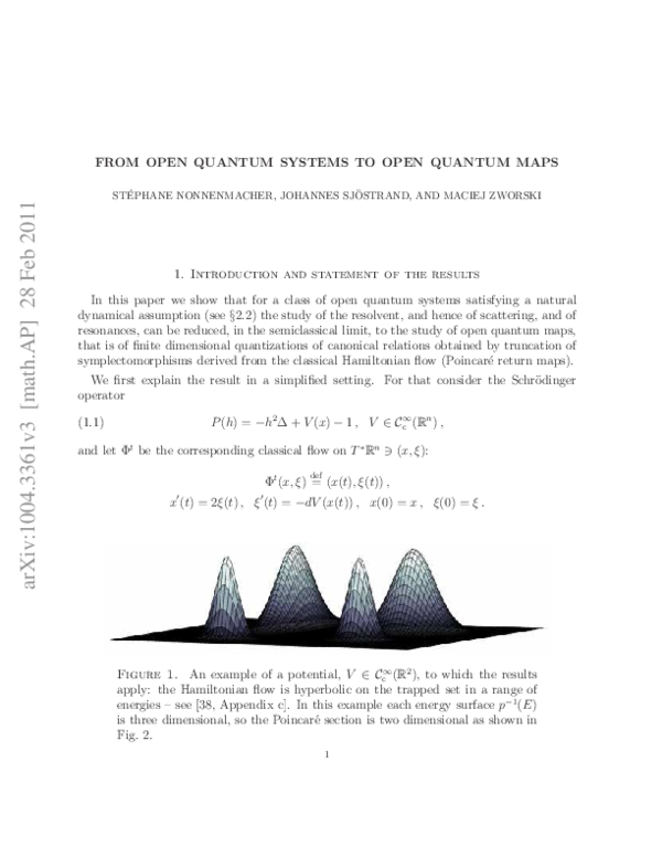
 Stéphane Nonnenmacher