EPJ manuscript No. (will be inserted by the editor) Sum of exit times in a series of two metastable states Emilio N.M. Cirillo1,a , Francesca R. Nardi2,b , and Cristian Spitoni3,c 1 2 3 Dipartimento di Scienze di Base e Applicate per l’Ingegneria, Sapienza Università di Roma, via A. Scarpa 16, 00161 Roma, Italy Department of Mathematics and Computer Science, Eindhoven University of Technology, P.O. Box 513, 5600 MB Eindhoven, The Netherlands Department of Mathematics, Budapestlaan 6, 3584 CD Utrecht,The Netherlands Abstract. The problem of not degenerate in energy metastable states forming a series in the framework of reversible finite state space Markov chains is considered. Metastability has been widely studied both in the mathematical and physical literature. Metastable states arises close to a first order phase transition, when the system can be trapped for a long time (exponentially long with respect to the inverse of the temperature) before switching to the thermodynamically stable phase. In this paper, under rather general conditions, we give a sharp estimate of the exit time from a metastable state in a presence of a second metastable state that must be necessarily visited by the system before eventually reaching the stable phase. In this framework we give a sharp estimate of the exit time from the metastable state at higher energy and, on the proper exponential time scale, we prove an addition rule. As an application of the theory, we study the Blume–Capel model in the zero chemical potential case. 1 Introduction Metastable states in finite volume Statistical Mechanics lattice systems, in which stochastic transition between states are controlled by an energy function, is a well understood phenomenon. Different mathematical theories have been developed in the last decades. The pioneering pathwise approach [1–3], further developed for non– reversible dynamics in [4], and the more recent potential theoretic approach [5–7], further developed in [8] via the use of the trace process, allow a thorough description of the phenomenon. The first theory gives a handy definition of the metastable state and a physically clear interpretation of the associated exit time. In the low temperature limit, it has been proven indeed that the time scale on which the system leaves the metastable state is exponentially large with the inverse temperature, with a mass given by the smallest energy barrier that the system has to overcome along the paths connecting a b c e-mail: emilio.cirillo@uniroma1.it e-mail: F.R.Nardi@tue.nl e-mail: C.Spitoni@uu.nl 2 Will be inserted by the editor the metastable state to the stable state. Moreover, the theory gives information about the paths followed by the system during its transition to the stable state. In particular it ensures that with high probability the system visits one of the configurations, namely, the critical droplets, where the smallest energy barrier is attained before reaching the stable state. The latter theory, on the other hand, allows a precise estimate of the mean exit time. In particular it is proven that, measured in terms of the exponential time scale, such a mean time can be written in terms of a quantity, called capacity, which can be bounded from above and from below by using effective variational principles. Under suitable hypotheses on the energy landscape, the theory allows the computation of the prefactor and, what is very relevant on physical grounds, shows that it does depend on entropic effects. Indeed, in many specific models the prefactor has been computed explicitly and it turns out to be connected, loosely speaking, to the number of possible ways in which the system can perform its transition to the stable state [1, 9]. More precisely, it depends on the number of critical droplets that the system can use as a gate towards the stable state. In this framework general results are proven under suitable hypotheses on the energy landscape ruling out the possibility to have multiple non degenerate in energy metastable states. In this paper we approach precisely such a problem and assume that two metastable states are indeed present. Moreover, we chose a peculiar structure of the energy landscape such that the two states form a “series”, in the sense that, starting from the metastable state at higher energy, the system has to visit necessarily (in probability in the low temperature limit) the second one in its way towards the ground state. We prove a sort of addition rule for the exit time and compute, on the exponential scale, a sharp estimate for the exit time. We approach this problem in the framework of rather general reversible Markov chains. Our aim is that of introducing a model covering both the standard Statistical Mechanics stochastic lattice models (e.g., the Metropolis dynamics) and the reversible Probabilistic Cellular Automata. In this framework we assume a minimal characterization of the energy landscape sufficient to ensure both the presence of two non degenerate in energy metastable state and their serial structure. In the last part of the paper we discuss an application of this theory. Indeed, we approach the Blume–Capel model [10, 11], whose metastability behavior has already been studied from different point of views and in different limits in [12–15], and we discuss how to derive, with a different method, the same result recently proven in [14] on the sharp estimate of the exit time from the metastable minus one state in the zero chemical potential case. We mention that the application of our results to the Probabilistic Cellular Automaton studied in [16] is reported in [17]. The paper is organized as follows: in Section 2 the general model is introduced and our main results are stated. Those results are then proved in Section 3. Finally, the application to the Blume–Capel model is discussed in Section 4. 2 Model and results In this section we first introduce a general reversible Markov chain and specify the conditions on the energy landscape in order to have a series of metastable states. We next state our main results in this framework. 2.1 Reversible Markov chains We want to give the notion of reversible Markov chain [3, Condition R, page 335] in a quite general setup so that the theory will apply to different and relevant examples Will be inserted by the editor 3 such as Statistical Mechanics Lattice models and the reversible Probabilistic Cellular Automata. Consider a finite state space X and a family of irreducible and aperiodic Markov chain x(t), with t ∈ Z+ parametrized by the parameter β > 0, called inverse temperature. We let pβ (x, y) and µβ (x), for x, y ∈ X be respectively the transition matrix and the stationary measure. We assume that the Markov chains are reversible with respect to µβ , namely, µβ (x)pβ (x, y) = pβ (y, x)µβ (y) (1) for any x, y ∈ X. We also assume that if a jump is not allowed, that does not depend on β, namely, if pβ ′ (x, y) = 0 then pβ ′′ (x, y) = 0 for any β ′′ . The definition of the model will be completed by assuming a slightly enforced version of the well known Wentzel–Friedlin condition and by requiring that the stationary measure is “close” to a Gibbs one1 . More precisely, we assume that there exists ∆ : X × X → R+ ∪ {∞} and r : X × X → R such that, for any x, y ∈ X, ∆(x, y) = ∞ if pβ (x, y) = 0 and lim [− log pβ (x, y) − β∆(x, y)] = r(x, y) if pβ (x, y) > 0. β→∞ (2) Note that ∆ and r do not depend on the inverse temperature. We shall call ∆ the cost function. Moreover, we assume that there exist two functions s, H : X → R and a family of functions Gβ : X → R parametrized by β > 0 such that µβ (x) = P 1 e−Gβ (x) and −Gβ (y) y∈X e lim [Gβ (x)) − βH(x)] = s(x) β→∞ (3) for x ∈ X and maxx∈X s(x) = s̄ < ∞. The normalization factor in µβ is denoted by Zβ and called partition function. Note that the function H does not depend on the inverse temperature. We shall call H the Hamiltonian or energy of the model. From (2) and (3) it follows immediately that lim β→∞ 1 log pβ (x, y) = −∆(x, y) β for all x, y ∈ X such that pβ (x, y) > 0 and lim β→∞ 1 Gβ (x) = H(x) β for x ∈ X. From (1) and the conditions above it follows also that H(x) + ∆(x, y) = ∆(y, x) + H(y) (4) for all x, y ∈ X. For any x ∈ X, we denote by Px (·) and Ex [·] respectively the probability and the average along the trajectories of the process started at x. 1 The fact that the stationary measure is close to a Gibbs one at low temperature is generally valid in the framework of Wentzell–Freidlin dynamics, see, e.g., [18, Proposition 4.1]. What we assume in this paper, see (3), is, on the other hand, slightly stronger. 4 Will be inserted by the editor 2.2 Examples In this section we discuss two important examples of dynamics fitting in the general scheme depicted above. The Metropolis dynamics on the states space X with energy K : X → R, inverse temperature β, and connection matrix q(x, y) is defined by letting pβ (x, y) = q(x, y) e−β[K(y)−K(x)]+ if x 6= y where, for any real a, we let [a]+ = a if a > 0 and [a]+ = 0 otherwise be the positive part of a, and X pβ (x, x) = 1 − pβ (x, y). y6=x It is well known that the Metropolis dynamics has as stationary measure the Gibbs measure with Hamiltonian K, so that the condition (3) is satisfied with Gβ = βK and s = 0. Now, we let r(x, x) = 0 and r(x, y) = − log q(x, y) for x 6= y and q(x, y) > 0. For any x 6= y, we let also ∆(x, y) = ∞ if q(x, y) = 0 and ∆(x, y) = [K(y) − K(x)]+ otherwise. Finally, we let ∆(x, x) = ∞ if pβ (x, x) = 0 and ∆(x, x) = −(1/β) log pβ (x, x) otherwise. It is immediate to verify that condition (2) is satisfied for any x, y ∈ X. A second important example is that of reversible Probabilistic Cellular Automata (PCA). Reversible PCA have been introduced in [19], see also [20] for a detailed discussion, and provide a very interesting example of dynamics with a parallel updating rule which are reversible with respect to a stationary measure which is very close to a Gibbs measure. The metastable behavior of some reversible Probabilistic Cellular Automata has been firstly studied in [21]. Let Λ ⊂ Z2 be a finite cube with periodic boundary conditions. Associate with each site i ∈ Λ the state variable xi ∈ {−1, +1} and denote by X = {−1, +1}Λ the state space. For any x ∈ X we consider on {−1, +1} the probability measure io h X 1n k(j)xj + h 1 + s tanh β fx,β (s) = 2 j∈Λ for s ∈ {−1, +1}, where β > 0 and h ∈ R are called inverse temperature and magnetic field respectively. The function k : Z2 → R is such that its support is a subset of Λ and k(j) = k(−j) for all j ∈ Λ. Recall that, by definition, the support of the function k is the subset of Λ where the function k is different from zero. We assume, also, that X k(j − i)xj + h 6= 0 (5) j∈Λ for any x ∈ X and i ∈ Λ. We finally introduce the shift Θi on the torus, for any i ∈ Λ, defined as the map Θi : X → X such that (Θi x)j = xi+j . A reversible PCA is the Markov chain on X with transition matrix Y fΘi x,β (yi ) pβ (x, y) = i∈Λ for x, y ∈ X. We remark that the character of the evolution is parallel, in the sense that at each time all the spins are potentially flipped. It is not difficult to prove [19] that the above specified PCA dynamics is reversible with respect to the finite–volume Gibbs–like measure µβ (x) = 1 −Fβ (x) e Zβ Will be inserted by the editor with Fβ (x) = −βh X xi − i∈Λ X i∈Λ 5 i h X k(j − i)xj + h log cosh β j∈Λ with Zβ the normalization constant. The low–temperature behavior of the stationary measure of the PCA can be guessed by looking at the function X X X 1 k(j − i)xj + h xi − Fβ (x) = −h β→∞ β K(x) = lim i∈Λ j∈Λ i∈Λ The difference between Fβ and βK can be computed explicitly, indeed in [20] it is proven that  n o X X k(j − i)xj + h log 1 + exp − 2β Fβ (x) − βK(x) = − + |Λ| log 2 j∈Λ i∈Λ for each β > 0 and x ∈ X. From the remarks above, recall also the assumption (5), it follows immediately that the reversible PCA satisfies condition (3) with Gβ = Fβ , H = K, and s(x) = |Λ| log 2 for any x ∈ X. As for the transition rates, we set X 1 log pβ (x, y) = β→∞ β i∈Λ: V (x, y) = − lim yi ( P 2 j∈Λ k(j−i)xj +h)<0 X k(j − i)xj + h j∈Λ We shall prove that X − log pβ (x, y) − βV (x, y) = log(1 + e−2β| P j∈Λ k(j−i)xi +h| ) (6) i∈Λ Thus, the reversible PCA satisfies condition (2) with ∆ = V and r(x, y) = 0 for any x, y ∈ X. For completeness, we finally prove (6). In the following computation we shall use many times the assumption (5). First note that P X log(1 + e−2βyi [ j∈Λ k(j−i)xj +h] ) − log pβ (x, y) − βV (x, y) = i∈Λ  X X k(j − i)xj + h 2yi +β yi ( P j∈Λ i∈Λ: j∈Λ k(j−i)xj +h)<0 Hence X − log pβ (x, y) − βV (x, y) = log(1 + e−2βyi [ P j∈Λ k(j−i)xj +h] ) i∈Λ: P yi ( j∈Λ k(j−i)xj +h)>0 X + yi ( P log(1 + e−2βyi [ P j∈Λ k(j−i)xj +h] i∈Λ: j∈Λ k(j−i)xj +h)<0 +β yi ( P X 2yi i∈Λ: j∈Λ k(j−i)xj +h)<0 X j∈Λ k(j − i)xj + h  ) 6 Will be inserted by the editor Finally, X − log pβ (x, y) − βV (x, y) = log(1 + e−2βyi [ i∈Λ: P yi ( j∈Λ k(j−i)xj +h)>0 + yi ( P X log(e2βyi [ P P j∈Λ j∈Λ k(j−i)xj +h] k(j−i)xj +h] ) + 1) i∈Λ: j∈Λ k(j−i)xj +h)<0 yielding (6). 2.3 Energy landscape After the short “intermezzo” on the Metropolis and the reversible PCA models, we come back to the general setup of Section 2.1. Let Q be the set of pairs (x, y) ∈ X ×X such that pβ (x, y) > 0 or, equivalently, ∆(x, y) < ∞. The quadruple (X, Q, H, ∆) is then a reversible energy landscape [12]. Given Y ⊂ X we let its external boundary ∂Y be the collection of states z ∈ X \ Y such that there exists y ∈ Y such that (y, z) ∈ Q. In words, the external boundary is made of those states outside Y such that there exists a state in Y where the system can jump. Given Y ⊂ X such that H(y) = H(y ′ ) for any y, y ′ ∈ Y , we shall denote by H(Y ) the energy of the states in Y . For any Y ⊂ X we shall denote by F (Y ) the set of the minima of the energy inside Y , that is to say y ∈ F (Y ) if and only if H(y ′ ) ≥ H(y) for any y ′ ∈ Y . We let Xs := F (X) be the set of ground states of H, namely, the set of the absolute minima of the energy. For any positive integer n, ω ∈ X n such that (ωi , ωi+1 ) ∈ Q for all i = 1, . . . , n − 1 is called a path joining ω0 to ωn ; we also say that n is the length of the path. For any path ω of length n, we let Φω := max i=1,...,n−1 [H(ωi ) + ∆(ωi , ωi+1 )] (7) be the height of the path2 . For any y, z ∈ X we denote by Ω(y, z) the set of the paths joining y to z. For any y, z ∈ X we define the communication height between y and z as Φ(y, z) := min Φω (8) ω∈Ω(y,z) From (4), (7), and (8) it follows immediately that Φ(y, z) = Φ(z, y) (9) for all y, z ∈ X. For any Y, Z ⊂ X we let Φ(Y, Z) := min ω∈Ω(Y,Z) Φω = min Φ(y, z) y∈Y,z∈Z (10) where we have used the notation Ω(Y, Z) for the set of paths joining a state in Y to a state in Z. For any y, z ∈ X we define also the communication cost from y to z as the quantity Φ(y, z) − H(y). Note that in general the communication cost from y to z differs from that from z to y. 2 Since the energy landscape is reversible, the energy of the state ωn is implicitly taken into account in (7), indeed (4) implies H(ωn ) ≤ ∆(ωn−1 , ωn ) + H(ωn−1 ). Will be inserted by the editor 7 2.4 Metastable states For any x ∈ X we denote by Ix the set of states y ∈ X such that H(y) < H(x). Note that Ix = ∅ if x ∈ Xs . We then define the stability level of any x ∈ X \ Xs Vx := Φ(x, Ix ) − H(x) ≥ 0 (11) Note that the stability level Vx of x is the minimal communication cost that, starting from x, has to be payed in order to reach states at energy lower than H(x). Following [1] we now introduce the notion of maximal stability level. Assume X \ Xs 6= ∅, we let the maximal stability level be Γm := sup Vx (12) x∈X\Xs Definition 1 We call metastable set Xm , the set Xm := {x ∈ X \ Xs : Vx = Γm } (13) Note that, since the state space is finite, the maximal stability level Γm is a finite number. Following [1], that is to say by assuming the so called pathwise point of view, we shall call Xm the set of metastable states of the system. Each state x ∈ Xm is called metastable. A different, even if strictly related, notion of metastable states is that given in [5] in the framework of the Potential Theoretic Approach. First recall that the Dirichlet form associated with the reversible Markov chain is defined as the functional Dβ [f ] := 1 X µβ (y)pβ (y, z)[f (y) − f (z)]2 2 (14) y,z∈X where f : X → R is a generic function. Thus, given two not empty disjoint sets Y, Z ⊂ X the capacity of the pair Y and Z can be defined as capβ (Y, Z) := min Dβ [f ] (15) f :X→[0,1] f |Y =1,f |Z =0 Note that the capacity is a symmetric function of the sets Y and Z. It can be proven that the right hand side of (15) has a unique minimizer called equilibrium potential of the pair Y and Z. A nice interpretation of the equilibrium potential in terms of hitting times can be given. For x ∈ X and Y ⊂ X we shall denote by τYx the first hitting time to Y of the chain started at x. Whenever possible we shall drop the superscript denoting the starting point from the notation. Then, it can be proven that the equilibrium potential of the pair Y and Z is equal to the function hY,Z defined as follows   Px (τY < τZ ) for x ∈ X \ (Y ∪ Z) for x ∈ Y hY,Z (x) = 1 (16) 0 for x ∈ Z where τY and τZ are, respectively, the first hitting time to Y and Z for the chain started at x. It can be also proven that, for any Y ⊂ X and z ∈ X \ Y , capβ (z, Y ) = µβ (z)Pz (τY < τz ) see [22, equation (3.10)]. (17) 8 Will be inserted by the editor Definition 2 A set M ⊂ X is said to be p.t.a.–metastable if lim β→∞ maxx∈M µβ (x)[capβ (x, M )] / −1 minx∈M µβ (x)[capβ (x, M \ {x})] −1 =0 (18) The prefix p.t.a. stands for potential theoretic approach. We used this expression in order to avoid confusion with the set of metastable states Xm introduced in (13). The physical meaning of the above definition can be understood once one remarks that the quantity µβ (x)/capβ (x, y), for any x, y ∈ X, is strictly related to the communication cost between the states x and y, see Proposition 1. Thus, condition (18) ensures that the communication cost between any state outside M and M itself is smaller than the communication cost between any two states in M . In other words, it states that getting to M starting from any state outside M is “much” easier than going from any point in M to any other point in M . Finally, given a p.t.a.–metastable set M ⊂ X, for any x ∈ M we let A(x) := {y ∈ X : Py (τx = τM ) = sup Py (τz = τM )} (19) z∈M be the valley associated with x. For any y ∈ X and any z ∈ M the quantity Py (τz = τM ) measures the probability that, starting from y, the system touches M for the first time in z. Thus, by computing supz,∈M Py (τz = τM ), one detects the best way to touch M for the system started at y. Hence, the condition Py (τx = τM ) = supz,∈M Py (τz = τM ) selects all the sites y such that, for the system started at y, the best way to touch M is that of touching it for the first time at x. 2.5 Series of metastable states The aim of this paper is that of proving an addition formula for the exit time from metastable states in the case in which they form a series. With this expression we mean that the structure of the energy landscape is such that the system has two non degenerate in energy metastable states and the system, started at the one having higher energy, must necessarily pass through the second one before relaxing to the stable state. See Fig. 1 for a schematic description of the situation we have in mind and that will be formalized through the following conditions. Condition 1 Recall (12) and (13).We assume that the energy landscape (X, Q, H, ∆) is such that there exist three states x2 , x1 , and x0 such that Xs = {x0 }, Xm = {x1 , x2 }, and H(x2 ) > H(x1 ). Note that, by recalling the definition of the set of ground states Xs , we immediately have that H(x1 ) > H(x0 ) (20) Moreover, from the definition (12) of maximal stability level it follows that (see [12, Theorem 2.3]) the communication cost from x2 to x0 is equal to that from x1 to x0 , that is to say Φ(x2 , x0 ) − H(x2 ) = Φ(x1 , x0 ) − H(x1 ) = Γm (21) Note that, since x2 is a metastable state, its stability level cannot be lower than Γm . Then, recalling that H(x2 ) > H(x1 ), one has that Φ(x2 , x1 ) − H(x2 ) ≥ Γm . On the other hand, (21) implies that there exists a path ω ∈ Ω(x2 , x1 ) such that Φω = H(x2 ) + Γm and, hence, Φ(x2 , x1 ) − H(x2 ) ≤ Γm . The two bounds finally imply that Φ(x2 , x1 ) − H(x2 ) = Γm (22) Will be inserted by the editor 9 ✻ ✻ Γ Γ ❄ x2 ❄ x1 x0 Fig. 1. Schematic description of the energy landscape for a series of metastable states. Note that the communication cost from x0 to x2 and that from x1 to x2 are larger than Γm , that is to say, Φ(x0 , x2 ) − H(x0 ) > Γm and Φ(x1 , x2 ) − H(x1 ) > Γm (23) Indeed, by recalling the reversibility property (9) we have Φ(x1 , x2 ) − H(x1 ) = Φ(x2 , x1 ) − H(x2 ) + H(x2 ) − H(x1 ) = Γm + H(x2 ) − H(x1 ) > Γm where in the last two steps we have used (22) and Condition 1, which proves the second of the two equations (23). The first of them can be proved similarly. We want to implement in the model the series structure depicted in Fig. 1. With this we mean that when the system is started at x2 with high probability it will visit x1 before x0 . For this reason we shall assume the following condition. Condition 2 Condition 1 is satisfied and lim Px2 (τx0 < τx1 ) = 0 β→∞ (24) We remark that the Condition 2 is indeed a condition on the equilibrium potential hx0 ,x1 evaluated at x2 . The most important goal of this paper is that of proving the formula (28) for the expectation of the escape time τx0 for the chain started at x2 . Such an expectation, hence, will be of order exp{βΓm } and the prefactor will be that given in (28). At the level of logarithmic equivalence, namely, by renouncing to get sharp estimate, this result can be proven by the methods in [1]. More precisely, one gets that (1/β) log Ex2 [τx0 ] tends to Γm in the large β limit. We can thus formulate the further assumptions that we shall need in the sequel in order to discuss the problem from the point of view of the Potential Theoretic Approach. Condition 3 Condition 1 is satisfied and there exists two positive constants k1 , k2 < ∞ such that µβ (x2 ) 1 = eβΓm [1 + o(1)], capβ (x2 , {x1 , x0 }) k2 µβ (x1 ) 1 = eβΓm [1 + o(1)] capβ (x1 , x0 ) k1 where o(1) denotes a function tending to zero in the limit β → ∞. (25) 10 Will be inserted by the editor 2.6 Main results We shall prove the addition rule for the exit times from the metastable states by using the sharp estimates provided by the Potential Theoretic Approach to metastability originally developed in [5]. Theorem 1 Assume Conditions 1 is satisfied. Then {x0 , x1 , x2 } ⊂ X is a p.t.a.– metastable set. By means of the theory in [5] it is possible to write asymptotic estimates of the first hitting time to a subset of a p.t.a.–metastable set when the dynamics is started in state of the same p.t.a.–metastable set not belonging to the considered subset. These results, see for instance [5, Theorem 1.3], are typically proven under suitable not degeneracy conditions [5, Definition 1.2] that are not satisfied in our case, due to the presence of multiple metastable states. In the following theorem we state two results that, for the reasons outlined above, can be deduced directly from those in [5]. On the other hand, as we shall discuss in detail in Section 3, they can be deduced by some of the results proven in [22] (see, also, [6]). But, since we assumed strong hypotheses on the energy landscape of the model, it will be possible to prove the theorem directly by means of simple estimates. This “ad hoc” proof is also given in Section 3. Theorem 2 Assume Conditions 1 is satisfied. Then Ex2 [τ{x1 ,x0 } ] = µβ (x2 ) µβ (x1 ) [1 + o(1)], Ex1 [τx0 ] = [1 + o(1)] capβ (x2 , {x1 , x0 }) capβ (x1 , x0 ) (26) Theorem 3 Assume Conditions 1 and 3 are satisfied. Then Ex2 [τ{x1 ,x0 } ] = eβΓm 1 [1 + o(1)] k2 and Ex1 [τx0 ] = eβΓm 1 [1 + o(1)] k1 Theorem 4 Assume Conditions 1, 2, and 3 are satisfied. Then 1 1 + [1 + o(1)] Ex2 [τx0 ] = eβΓm k1 k2 (27) (28) We remark that Theorem 4 gives an addition formula for the mean first hitting time to x0 starting from x2 . Neglecting terms of order o(1), such a mean time can be written as the sum of the mean hitting time to the pair {x1 , x0 } when the chain is started at x2 and of the mean hitting time to x0 when the chain is started at x1 . It is very interesting to note that no role is plaid in this decomposition by the mean hitting time to x1 for the chain started at x2 . Indeed, on the exp{βΓm } time scale no control can be proven for such a mean time. For instance, in the case of the Blume–Capel model that will be studied in Section 4, in [14, Proposition 2.5] it is proven that Ex2 [τx1 ]/eβΓm diverges in the limit β → ∞. 3 Proof of results In this section we proof the theorems stated above and related to the general setup given in Section 2.5. Proof of Theorem 1. The theorem follows immediately by Condition 1, (22), and [12, Theorem 3.6]. ⊔ ⊓ Will be inserted by the editor 11 We just note that the Theorem 3.6 in [12] has been proved in a slightly different context, but the proof given there applies also to the more general case studied here. Theorem 2 can be deduced by using the structure provided by Theorem 1 above, and the general results [22, Eq. (4.14) and Lemma 4.3]. Alternatively, one can use [6, Eq. (8.1.6), Eq. (8.3.3), and Lemma 8.13]. Since we assumed strong hypotheses on the energy landscape of the model, it is possible to prove directly equation (26) by means of simple estimates. Before discussing such a proof we state two useful lemmas. Recall Condition 1, in the first of the two lemmas we collect two bounds to the energy cost that has to be payed to go from any state x 6= x1 to x1 or to x0 . The second lemma is similar. Lemma 1 Assume Condition 1 is satisfied. For any x ∈ X and x 6= x1 . If H(x) ≤ H(x1 ), we have that Φ(x, x0 ) − H(x) < Γm and Φ(x, x1 ) − H(x1 ) ≥ Γm (29) Proof. Let us prove the first inequality. By Theorem 2.3 in [12] we have that Φ(x, x0 ) ≤ Γm + H(x). If by contradiction Φ(x, x0 ) = Γm + H(x) then, by the same Theorem 2.3 in [12], x ∈ Xm which is in contradiction with Condition 1. As regards the proof of the second inequality we distinguish two cases. Case H(x) < H(x1 ): we have that x ∈ Ix1 . By Definition 1 of metastable state and by (11), we get Φ(x1 , x) ≥ Φ(x1 , Ix1 ) = Γm + H(x1 ) that proves the inequality. Case H(x) = H(x1 ): let us define the set C := {y ∈ X : Φ(y, x1 ) < H(x1 ) + Γm } and show that x 6∈ C. Since H(x) = H(x1 ), the identity Ix = Ix1 follows. Furthermore, being x1 ∈ Xm , we have C ∩ Ix1 = ∅; hence, C ∩ Ix = ∅ as well. Moreover, if x ∈ C then Vx = Φ(x, Ix ) − H(x) ≥ H(x1 ) + Γm − H(x) = Γm . By the Definition 1, x would be a metastable state, in contradiction with Condition 1. Hence, since x 6∈ C, we have that Φ(x, x1 ) ≥ Γm + H(x1 ) that proves the inequality. the inequality. ⊔ ⊓ Lemma 2 Assume Condition 1 is satisfied. For any x ∈ X and x ∈ / {x2 , x1 , x0 }. If H(x) ≤ H(x2 ), we have that Φ(x, {x1 , x0 }) − H(x) < Γm and Φ(x, x2 ) − H(x2 ) ≥ Γm (30) Proof. Let us prove the first inequality. By Theorem 2.3 in [12] we have Φ(x, {x1 , x0 }) ≤ Φ(x, x0 ) ≤ Γm + H(x). If by absurdity Φ(x, x0 ) = Γm + H(x) then, by the same Theorem 2.3 in [12], x ∈ Xm which is in contradiction with Condition 1. As regards the proof of the second inequality we distinguish two cases. Case H(x) < H(x2 ): we have that x ∈ Ix2 . By Definition 1 of metastable state and by (11), we get Φ(x2 , x) ≥ Φ(x2 , Ix2 ) = Γm + H(x2 ) that proves the inequality. Case H(x) = H(x2 ): let us define the set C := {y ∈ X : Φ(y, x2 ) < H(x2 ) + Γm } 12 Will be inserted by the editor and show that x 6∈ C. Since H(x) = H(x2 ), the identity Ix = Ix2 follows. Furthermore, being x2 ∈ Xm , we have C ∩ Ix2 = ∅; hence, C ∩ Ix = ∅ as well. Moreover, if x ∈ C then Vx = Φ(x, Ix ) − H(x) ≥ H(x2 ) + Γm − H(x) = Γ . By the Definition 1, x would be a metastable state, in contradiction with Condition 1. Hence, since x 6∈ C, we have that Φ(x, x2 ) ≥ Γm + H(x2 ) ⊔ ⊓ that proves the inequality. Proof of Theorem 2. We prove in details the right of equation (26). The proof is based on Lemma 1. The equation on the left can be deduced with precisely the same arguments and using the bounds in Lemma 2. The only general results used is the representation of the expected mean time in terms of the Green function given in [5, Corollary 3.3] (see also equation (3.18) in the proof of the Theorem 3.5 in [5] or [23, Eq. (4.29)]). Indeed, recalling (17) above, we have: Ex1 [τx0 ] = X 1 µβ (x) hx1 ,x0 (x) capβ (x1 , x0 ) (31) x∈X Considering the contribution of x1 in the sum and recalling (16), we get the following lower bound: Ex1 [τx0 ] ≥ 1 1 µβ (x1 )hx1 ,x0 (x1 ) = µβ (x1 ) cap(x1 , x0 ) cap(x1 , x0 ) (32) In order to provide un upper bound, we first use the boundary conditions in (16) to rewrite (31) as follows: i h X X 1 µβ (x)hx1 ,x0 (x) Ex1 [τx0 ] = µβ (x)hx1 ,x0 (x) + cap(x1 , x0 ) x∈X\x , x∈X\x , 0 H(x)>H(x1 ) 0 H(x)≤H(x1 ) Recalling that hx1 ,x0 (x1 ) = 1, the equilibrium potential is not bigger than one, the configuration space is finite, and µβ (x) = µβ (x1 ) exp{−βδ} for some positive δ and for any x ∈ X such that H(x) > H(x1 ), we get i h X 1 Ex1 [τx0 ] = (33) µβ (x) hx1 ,x0 (x) + µβ (x1 )[1 + o(1)] cap(x1 , x0 ) x∈X\x , 0 H(x)≤H(x1 ), x6=x1 By (16) and (2) we can give the following upper bound for the equilibrium potential hx1 ,x0 (x), for any x 6= x1 , x0 hx1 ,x0 (x) ≤ cap(x, x1 ) . cap(x, x0 ) Thus, if H(x) ≤ H(x1 ), we have hx1 ,x0 (x) ≤ C e−β(Γm +H(x1 )) µβ (x1 ) e−βΦ(x,x1 ) ≤ C = Ce−βδ −βΦ(x,x ) −β(Γ +H(x)−δ) 0 m µβ (x) e e where in the first inequality we used Proposition 1, in the second Lemma 1, and C, δ are suitable positive constants. By using (33) we get Ex1 [τx0 ] ≤ h 1 cap(x1 , x0 ) X Cµβ (x)e−βδ x∈X\x0 , H(x)≤H(x1 ), x6=x1 i µβ (x1 ) + µβ (x1 )[1 + o(1)] µβ (x) Will be inserted by the editor 13 Which implies Ex1 [τx0 ] ≤ µβ (x1 ) [1 + o(1)] cap(x1 , x0 ) (34) where we have used that the configuration space is finite. The Theorem finally follows by (32) and (34). ⊔ ⊓ Proof of Theorem 3. The theorem follows immediately by exploiting Condition 3 and applying Theorem 2. ⊔ ⊓ The proof of Theorem 4 is based on the following lemma. Lemma 3 Given three states y, w, z ∈ X pairwise mutually different, we have that the following holds Ey [τz ] = Ey [τ{w,z} ] + Ew [τz ]Py (τw < τz ) (35) Proof. First of all we note that Ey (τz ) = Ey [τz Iτw <τz ] + Ey [τz Iτw ≥τz ] We now rewrite the first term as follows Ey [τz I{τw <τz } ] = Ey [Ey [τz I{τw <τz } |Fτw ]] = Ey [I{τw <τz } (τw + Ew [τz ])] = Ey [τw I{τw <τz } ] + Py (τw < τz )Ew (τz ). where we have used the fact that τw is a stopping time, that I{τw <τz } is measurable with respect to the pre–τw –σ–algebra Fτw and the strong Markov property which gives Ey [τz |Fτw ] = τw + Ew [τz ] on the event {τw ≤ τz }. Since (τw I{τw <τz } + τz I{τw ≥τz } ) = τ{w,z} , (35) follows. ⊔ ⊓ Proof of Theorem 4. By (35) we have that Ex2 [τx0 ] = Ex2 [τ{x1 ,x0 } ] + Ex1 [τx0 ]Px2 (τx1 < τx0 ) By Theorem 3 and Condition 2 it follows that   1 1 βΓm + [1 + o(1)] Ex2 [τx0 ] = e k1 k2 which completes the proof. ⊔ ⊓ 4 Application to the Blume–Capel model In this section, as a possible application of the theory described above, we apply our results to the case of the Blume–Capel model [10, 11]. In particular, we consider the model with null chemical potential, which has two metastable states non degenerate in energy. We shall then derive, in a different way, the results already appeared in [14]. Let us consider a square lattice Λ ⊂ Z2 with periodic boundary conditions and side length L. Let {−1, 0, +1} be the single spin state space and X := {−1, 0, +1}Λ be the configuration space. The Hamiltonian of the model [12] is X X H(σ) = σ(i) (36) (σ(i) − σ(j))2 − h hi,ji i∈Λ 14 Will be inserted by the editor ℓc −1 ℓc −1 mi ℓc r ze os nu s ze es ℓc Pc ℓc −1 p lu se s ro ℓc −1 mi s ℓc r ze s oe nu s ze es ℓc p lu Pc ′ Qc ro s se s Qc ′ Fig. 2. Schematic representation of the configurations Pc and Qc . The protuberance can be either on the left or on the right vertical edge (the longest ones in the picture) and there it can be shifted freely. Note that the two configurations Pc ′ and Qc ′ , with the protuberance on the shortest side, do not play any role in the transition from the metastable to the stable state. for any σ ∈ X , where the first sum runs over the pairs of nearest neighbors and h ∈ R is the magnetic field. We denote by µβ the corresponding Gibbs measure X exp{−βH(η)} µβ (σ) = exp{−βH(σ)}/ η∈X with inverse temperature β. We shall study the zero chemical potential Blume–Capel model for the following choice of the parameters: the magnetic field h and the torus Λ are such that 0 < h < 1, 2/h is not integer, and |Λ| ≥ 49/h4 finite, where, for any positive real a, we let ⌊a⌋ be the largest integer smaller than or equal to a. The time evolution of the model is defined by the Metropolis Markov chain σt with t = 0, 1, . . . the discrete time variable, see Section 2.2, with Hamiltonian H and connectivity matrix  0 if σ, η differ at more than one site q(σ, η) := . 1/(2|Λ|) otherwise As already remarked in Section 2.2, the dynamics above is an example of the dynamics defined in Section 2.1, provided we let i) r(x, x) = 0 and r(x, y) = − log q(x, y) for x 6= y and q(x, y) > 0; ii) for any x 6= y, ∆(x, y) = ∞ if q(x, y) = 0 and ∆(x, y) = [H(y) − H(x)]+ otherwise; iii) ∆(x, x) = ∞ if pβ (x, x) = 0 and ∆(x, x) = −(1/β) log pβ (x, x) otherwise. The notation introduced in Section 2.1–2.4 is then trivially particularized to the Blume–Capel case. Given V ⊂ Λ and σ ∈ X , we let σV be the restriction of σ to V , namely, σV ∈ {−1, +1}V such that σV (i) = σ(i) for any i ∈ V . We let u ∈ X to be the configuration such that u(i) = +1 for all i ∈ Λ. Other two very relevant configurations are d and 0, that is the configuration in which all the spin are minus one and the one in which all the spins are zero. Note that in these configurations the exchange part of the energy is minimal, although the magnetic part is not. 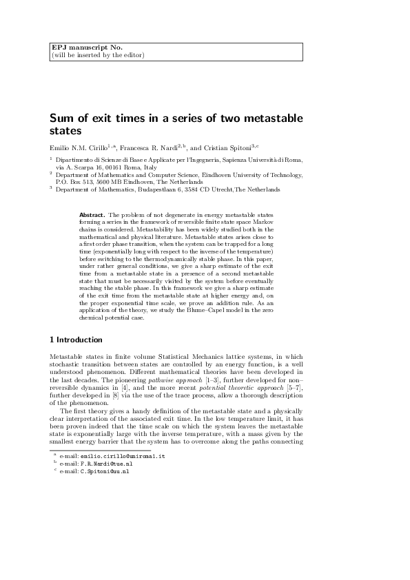We now define the critical length of the model as j2k +1 (37) ℓc := h We denote by Pc the set of configurations in which all the spins are minus excepted those, which are zeros, in a rectangle of sides long ℓc and ℓc − 1 and in a site adjacent to one of the longest sides of the rectangle (see Fig. 2). We denote by Qc the set of configurations in which all the spins are zeros excepted those, which are pluses, in a rectangle of sides long ℓc and ℓc − 1 and in a site adjacent to one of the longest sides of the rectangle (see the caption of Fig. 2). We have: H(Pc ) − H(d) = H(Qc ) − H(0) = 4ℓc − h[ℓc (ℓc − 1) + 1] Will be inserted by the editor 15 We then set Γc := H(Pc ) − H(d) = H(Qc ) − H(0) A simple direct computation shows that for h small one has Γc ∼ 4/h. In order to give a result in the spirit of Theorem 4 in the case of the Blume– Capel model, we first have to prove preliminary Lemmas ensuring that the Conditions assumed in the general discussion in Section 2.5 are satisfied in the Blume–Capel case. Lemma 4 With the parameters chosen as below (36), we have that Xs = {u}, Xm = {d, 0}, and H(d) > H(0). Moreover, the maximal stability level Γm is equal to Γc . Lemma 5 With the parameters chosen as below (36), we have that there exists κ > 0 and β0 > 0 such that for any β > β0 Pd (τu < τ0 ) ≤ e−βκ (38) Lemma 6 With the parameters chosen as below (36), we have that 3eβΓc µβ (0) 3eβΓc µβ (d) = [1 + o(1)], = [1 + o(1)] capβ (d, {0, u}) 2(2ℓc − 1) capβ (0, u) 2(2ℓc − 1) (39) For shortness we skip the proof of the model dependent results in Lemmas 4–6 that, altough not straitghforward, can be achieved by methods similar to those developed for the Ising model (see, arXiv:1603.03483). We stress that analogous results have been proven in [14, Proposition 2.3] for the continuous time version of the same model. We finally state our main results about the sharp estimate in the exit time in the Blume–Capel model with zero chemical potential. Theorem 5 With the parameters chosen as below (36), we have that Ed [τ{0,u} ] = eβΓc 3 3 [1 + o(1)], E0 [τu ] = eβΓc [1 + o(1)] 2(2ℓc − 1) 2(2ℓc − 1) (40) Theorem 6 With the parameters chosen as below (36), we have that Ed [τu ] = eβΓc 3 [1 + o(1)] (2ℓc − 1) (41) The proof of the theorems is achieved by applying the general results discussed in Section 2.6 and the model dependent lemmas given above. Indeed, Theorem 5 follows by Theorem 3 and Lemmas 4–6, whereas Theorem 6 follows by Theorem 4, and Lemmas 4–6. Aknowledgements. ENMC thanks ICMS (TU/e, Eindhoven), Eurandom (TU/e, Eindhoven), the Mathematics Department of Delft University, and the Mathematics Department of Utrecht University for kind hospitality. FRN and CS thank A. Bovier for many stimulating discussions. ENMC and FRN thank E. Scoppola and F. den Hollander for illuminating discussions. The authors thank A. Gaudilliere and M. Slowik for useful discussions and comments. 16 Will be inserted by the editor A General bounds In this appendix we summarize some general results whose statement and proof can already be found in the literature but, sometimes, in slightly different contexts. Proposition 1 ([24, Lemma 3.1.1]) Consider the Markov chain defined in Section 2.1. For every not empty disjoint sets Y, Z ⊂ X there exist constants 0 < C1 < C2 < ∞ such that C1 ≤ eβΦ(Y,Z) Zβ capβ (Y, Z) ≤ C2 (1) for all β large enough. Proof. The upper bound can be obtained by choosing f = IK(Y,Z) in (15) with K(Y, Z) := {x ∈ X \ Y : Φ(x, Y ) ≤ Φ(Y, Z)} For any pair u, v ∈ X such that u ∈ K(Y, Z) and v ∈ X \ K(Y, Z), we have that H(u) + ∆(u, v) ≥ Φ(Y, Z). In fact, if by absurdity it were H(u) + ∆(u, v) < Φ(Y, Z), it would be possible to construct a path ω starting at v and ending in Y such that Φω < Φ(Y, Z), which is in contradiction with v ∈ X \ K(Y, Z). Hence, by (14) and (15) X 1 Zβ capβ (Y, Z) ≤ Zβ Dβ [IK(Y ) ] = pβ (u, v)e−Gβ (u) 2 u∈K(Y,Z) v∈X\K(Y,Z) Recalling (2) and (3), we get that there exists C such that for β large enough X Ce−β[H(u)+∆(u,v)] Zβ capβ (Y, Z) ≤ u∈K(Y ) v∈X\K(Y ) Finally, the upper bound in (1) follows from the fact that H(u) + ∆(u, v) ≥ Φ(Y, Z) for any u ∈ K(Y, Z) and v ∈ X \ K(Y, Z). The lower bound can be proven by picking any path ω = (ω0 , ω1 , . . . , ωn ) that realizes the minimax in Φ(Y, Z) and ignore all the transitions that are not the path and using the same argument as in the proof of [Lemma 3.1.1, [24]]. An alternative proof can be given applying the Berman–Konsowa lemma [Proposition 2.4, [25]] which provides a complementary variational principle, in the sense that any test flow will give a lower bound. Hence, the lower bound can be obtained by picking any path ω = (ω0 , ω1 , . . . , ωn ), with ω0 ∈ Y , ωn ∈ Z, such that it realizes the minimax in Φ(Y, Z) and such that H(ωi ) + ∆(ωi , ωi+1 ) ≤ Φ(Y, Z) for i ∈ {0, . . . , n − 1} (recall (7) and (10)). If we choose a unitary flow for the edges in the path ω and null otherwise, the induced Markov chains is a deterministic chain along the path, so that the expectation in [Proposition 2.4, [25]] is just the contribution of the deterministic path. Hence, for the chosen flow we have: #−1 "n−1 X 1 −βΦ(Y,Z) 1 e [1 + o(1)] ≥ C1 capβ (Y, Z) ≥ µβ (ωk )pβ (ωk , ωk+1 ) Zβ k=0 where in the last inequality we used (2) and (3). ⊔ ⊓ Proposition 2 Consider the Markov chain defined in Section 2.1. We have that Py (τy1 < τy2 ) ≤ capβ (y, y1 ) capβ (y, y2 ) for any y 6= y1 , y1 6= y2 , y 6= y2 , and y, y1 , y2 ∈ X. (2) Will be inserted by the editor 17 Proof. Given y, y1 , y2 ∈ X, a renewal argument and the strong Markov property yield: Py (τy1 < τy2 ) = Py (τy1 < τy2 , τ{y1 ,y2 } > τy ) + Py (τy1 < τy2 , τ{y1 ,y2 } < τy ) = Py (τy1 < τy2 |τ{y1 ,y2 } > τy )Py (τ{y1 ,y2 } > τy ) +Py (τy1 < τy2 , τ{y1 ,y2 } < τy ) = Py (τy1 < τy2 )Py (τ{y1 ,y2 } > τy ) + Py (τy1 < τy2 , τy1 < τy ) = Py (τy1 < τy2 )Py (τ{y1 ,y2 } > τy ) + Py (τy1 < τ{y2 ,y} ) Therefore Py (τy1 < τy2 ) = Py (τy1 < τ{y2 ,y} ) Py (τy1 < τ{y2 ,y} ) Py (τy1 < τy ) = ≤ 1 − Py (τ{y1 ,y2 } > τy ) Py (τ{y1 ,y2 } < τy ) Py (τy2 < τy ) Recalling (17), we can rewrite the ratio in terms of ratio of capacities: capβ (y, y1 ) Py (τy1 < τy ) = Py (τy2 < τy ) capβ (y, y2 ) Hence, we get (2). ⊔ ⊓ References 1. F. Manzo, F.R. Nardi, E. Olivieri, E. Scoppola, Journ. Stat. Phys. 115, (2004) 591–642. 2. E. Olivieri, E. Scoppola, Journ. Stat. Phys. 79, (1995) 613–647. 3. E. Olivieri, M.E. Vares, Large deviations and metastability (Cambridge University Press, UK, 2004). 4. E.N.M. Cirillo, F.R. Nardi, J. Sohier, Journ. Stat. Phys. 161, (2015) 365–403. 5. A. Bovier, M. Eckhoff, V. Gayrard, M. Klein, Comm. Math. Phys. 228, (2002) 219–255. 6. A. Bovier, F. den Hollander, Metastability: a potential–theoretic approach (Grundlehren der mathematischen Wissenschaften, Springer, 2015). 7. M. Slowik, Metastability in Stochastic Dynamics: Contributions to the Potential Theoretic Approach (ISBN-13: 978-3838134123, Südwestdeutscher Verlag für Hochschulschriften August 31, 2012). 8. J. Beltrán, C. Landim, Journ. Stat. Phys. 140, (2010) 1065–1114. 9. A. Bovier, F. Manzo, Journ. Stat. Phys. 107, (2002) 757–779. 10. M. Blume, Phys. Rev. 141, (1966) 517. 11. H.W. Capel, Physica 32, (1966) 966. 12. E.N.M. Cirillo, F.R. Nardi, Journ. Stat. Phys. 150, (2013) 1080–1114. 13. E.N.M. Cirillo, E. Olivieri, Journ. Stat. Phys. 83, (1996) 473–554. 14. C. Landim, P. Lemire, Journ. Stat. Phys. 164, (2016) 346–376. 15. F. Manzo, E. Olivieri, Journ. Stat. Phys. 104, (2001) 1029–1090. 16. E.N.M. Cirillo, F.R. Nardi, Journ. Stat. Phys. 110, (2003) 183–217. 17. E.N.M. Cirillo, F.R. Nardi, C. Spitoni, Sum of exit times in a series of two metastable states in Probabilistic Cellular Automata, Cellular Automata and Discrete Complex Systems, 22nd IFIP WG 1.5 International Workshop, AUTOMATA 2016, Zurich, Switzerland, June 15-17, 2016, Proceedings, Springer (2016). 18. O. Catoni. Simulated annealing algorithms and Markov chains with rare transitions, in Séminaire de Probabilités, XXXIII, volume 1709 of Lecture Notes in Math., pages 69–119. Springer, Berlin, 1999. 19. G. Grinstein, C. Jayaprakash, Y. He, Phys. Rev. Lett. 55, (1985) 2527–2530. 20. E.N.M. Cirillo, P.–Y. Louis, W. Ruszel, C. Spitoni, Automata.” Chaos, Solitons, and Fractals 64, (2014) 36–47. 21. S. Bigelis, E.N.M. Cirillo, J.L. Lebowitz, E.R. Speer, Phys. Rev. E 59, (1999) 3935. 18 Will be inserted by the editor 22. A. Bovier, Metastability: a potential theoretic approach Proceedings of ICM 2006, EMS Publishing House, 2006, pp. 499–518. 23. A. Gaudillière, Condenser physics applied to Markov Chains, XII Escola Brasileira de Probabilidade, Ouro Preto, Minas Gerais, Brazil, 2008. 24. A. Bovier, F. den Hollander, and F.R. Nardi, Probab. Theory Relat. Fields 135, (2006) 265–310. 25. A. Bovier, F. den Hollander and C. Spitoni, Ann. Prob. 38, (2010) 661–713.