Using Residual Times To Meet Deadlines In M/G/C Queues
Sarah Tasneem, Lester Lipsky, Reda Ammar, and Howard Sholl
CSE Department
University of Connecticut
Storrs, CT- 06269-1155
sarah, lester, reda, hasc@engr.uconn.edu
Abstract
In systems where customer service demands are only known probabilistically, there is very little to
distinguish between jobs. Therefore, no universal optimum scheduling strategy or algorithm exists. If the
distribution of job times is known, then the residual time (expected time remaining for a job), based on the
service it has already received, can be calculated. In a detailed discrete event simulation, we have explored
the use of this function for increasing the probability that a job will meet its deadline. We have tested many
different distributions with a wide range of σ 2 and shape, four of which are reported here. We compare
with RR and FCFS, and find that in all distributions studied our algorithm performs best. We also studied
the use of two slow servers versus one fast server, and have found that they provide comparable
performance, and in a few cases the double server system does better.
1. Introduction
There have been innumerable papers written on how to optimize performance in queueing
systems. They cover any number of different goals and conditions. From our point of view they
fall into two categories (with many possibilities in between):
(1) The service demand of each customer is known, and;
(2) The service demands of the individual customers are not known,
but the probability distribution function (pdf) of those demands is presumed to be known. So, for
instance, the mean and variance over all customers might be known, even though the time needed
by a particular customer is not known until that customer is finished.
Within each of these categories there are many possible goals. For instance, the goal might
be to minimize the system time, as in job processing in computer systems, or minimize the waiting
time, as in setting up telecommunication links. However, both of these would be useless in
situations where there are critical deadlines, as would be the case in airport security lines, where it
would be more important to maximize the fraction of passengers who get through in time to catch
their flights.
In this paper we consider the second category with the goal of maximizing the fraction of
jobs that meet their deadline. We compare several queueing disciplines for systems with Poisson
customer arrivals to a service station, with a given service time distribution. The distributions we
consider include: Uniform, Erlangian-3, Exponential, two hyper exponentials with the same
variance, and a four hyper-Erlangian, also with that variance. We also compare the performance
of single and double server systems with the same maximal capacity. Our method of evaluation is
1
by discrete event simulation. Comparison is made with analytic results that are available [Lip92,
BCM75].
Our particular research contribution is in using residual times as a criterion for selecting
customers for immediate service. The other service disciplines we consider are: FCFS, RoundRobin (RR). FCFS discipline is used in present day routers [RKB03]. It is interesting that these
disciplines have all been studied in the context of mean system time and have been shown to have
the same mean as that for the M/M/1 queue for all service time distributions [BCM75]. When
C 2 > 1 , RR outperforms FCFS. If C 2 < 1 , one should stick to FCFS. The famous PollaczekKhinchin formula gives the mean system time for FCFS M/G/1 , which has been tabulated in Table
1. Even though, different system time distributions may have the same mean and variance (and
thus the same system time for jobs), they may have different qualities for meeting deadlines. As far
as we know, this aspect has not been studied previously.
In this paper we have developed a dynamic scheduling algorithm for real time tasks using
task residual execution time, rm (t ) . By definition, rm (t ) is the expected remaining execution time
of a task after receiving a service time of t time units. In summary, our Residual Time Based
(RTB) algorithm provides a higher percentage of deadline makers than any of the other disciplines
considered, but at the expense of holding up a few customers much longer. Our results also show
that for some distributions, two slow processors are at least marginally better than one fast
processor.
The rest of the paper is organized as follows. In Section 2 we discuss the related works.
Following in Section 3, is a mathematical description what is meant by residual times and of the
different distributions used, and how we generate random samples from each of them. In Section 4
we explicitly describe our prototype scheduling system, together with our algorithm for using
residual times. In Section 5 we present the results we have at this time, and discuss their
implications. Finally, in Section 7 we draw the conclusions of the paper.
Note: The word, task, job and process are used interchangeably in the document.
2. Related Works
2.1. The Task Scheduling Problem
Given the enormous amount of literature available on scheduling, any survey can only
scratch the surface. Moreover, a large number of scheduling approaches are used upon radically
different assumptions making their comparison on a unified basis a rather difficult task [CK88,
SR94]. At the highest level the scheduling paradigm may be divided into two major categories:
real time and non real time. Within each of the categories scheduling techniques may also vary
depending on whether one has a precise knowledge of task execution time or the pdf.
2.1.1. Scheduling in Non Real time Systems
In the non real time case the usual objective is to minimize the total execution time of a
program and increase the overall throughput of the system. Topcouglo et al., provides a
classification of the proposed algorithms [THW02]. The algorithms are classified into a variety of
categories such as, list-scheduling algorithms [KA96] clustering algorithms [YG94], duplicationbased algorithms [AK94] and guided random search methods. Genetic Algorithms (GAs)
[HAR94] are one of the widely studied guided random search techniques for the task scheduling
problem. Although they provide a good quality of schedules, the execution time of Genetic
Algorithms is significantly higher than the other alternatives.
2
Several researchers have studied the problem of scheduling, which is known to be NPcomplete in its general form, when the program is represented as a task graph [THW02]. The
execution time of any task and the communication cost between any pair of processors is
considered to be one time unit. Thus, they have considered only deterministic execution time.
Adam et al. [ACD74] studied both deterministic and stochastic models for task execution time and
made a comparison of different list scheduling algorithms. For the latter, task execution is limited
to the uniform distribution.
Kwok and Ahmed [KA99] focused on taxonomy of DAG scheduling algorithms based on a
static scheduling problem, and are therefore only partial. Some algorithms assume the
computational cost of all the tasks to be uniform. This simplifying assumption may not hold in
practical situations. It is not always realistic to assume that the task execution times are uniform.
Because the amount of computations encapsulated in tasks are usually varied. Others do not
specify any distribution for task execution time. They just assume any arbitrary value.
2.1.2. Scheduling in Real time Systems
Scheduling algorithm in RT applications can be classified along many dimensions. For
example: periodic tasks, pre-emptable non-pre-emptable. Some of them deal only with periodic
tasks while others are intended only for a-periodic tasks. Another possible classification ranges
from static to dynamic. Ramamaritham and Stankovic [RS94] discuss several task scheduling
paradigms and identify several classes of scheduling algorithms.
A majority of scheduling algorithms reported in the literature, perform static scheduling
and hence have limited applicability since not all task characteristics are known a priori and further
tasks arrive dynamically. Recently many scheduling algorithms [RSS90] have been proposed to
dynamically schedule a set of tasks with computation times, deadlines, and task requirements.
Each task is characterized by its worst-case computation time deadline, arrival time and ready time.
Ramamritham in [R95] discusses a static algorithm for allocating and scheduling subtasks
of periodic tasks across sites in distributed systems. The computation times of subtasks represent
the worst-case computation time and are considered to be uniformly distributed between a
minimum (50 time unit) and maximum (100 time unit) value. It is assumed that the execution of
each subtask cannot be preempted. This way of selecting the execution time range (from 50 to 100)
reduces C 2 to a very small value (= 4/27), which the authors may not have realized.
Chetto and Chetto [CC89] considered the problem of scheduling hard periodic real time
tasks and hard sporadic tasks (tasks that arrive are required to be run just once [RS84]). In addition
to computation time and period, each periodic task is characterized by its dynamic remaining
execution time. But the authors have not mentioned how to obtain the remaining execution time in
a dynamic manner.
Liu and Layland [LL73] were perhaps the first to formally study priority driven
algorithms. They focused on the problem of scheduling periodic tasks on a single processor and
proposed two preemptive algorithms. The first one is called Rate-Monotonic (RM) algorithm,
which assigns static priorities to periodic tasks based on their periods. The second one is called the
Earliest Deadlines First (EDF), a dynamic priority assignment algorithm. The closer a tasks’
deadline, the higher the priority. This again is an intuitive priority assignment policy. EDF and RM
schedulers do not provide any quality of service (QoS) guarantee when the system is overloaded by
overbooking. Since, EDF [LL73] does not make use of the execution time of tasks, it is difficult to
mix non-real-time and real-time tasks effectively. Scheduling both real-time and non real-time
tasks under load requires knowing how long a real-time task is going to run [BMP98, NL97,
3
GGV96]. As a result, some new / different scheduling approach that addresses these limitations is
desirable. One can determine the latest time the task must start executing if one has the knowledge
of the exact time of how long a task will run. Thus, the scheduler may delay a job to start
executing in order to increase the number of jobs meeting deadlines. In this paper, we investigated
this issue and developed a dynamic scheduling strategy, which includes both the deadline and the
estimated execution time.
For dynamic scheduling with more than one processor, Mok and Destouzos [MD78] show
that an optimal scheduling algorithm does not exists. These negative results point out the need for
new approaches to solve scheduling problems in such systems. Those approaches may be different
depending on the job service time distribution (job size variability). In this paper we have
addressed this issue by running experiments for several distributions for both single and multiple
processor systems.
A job arrives with a service time and deadline requirement. As time evolves, both: (1) the
residual service time, depending on the amount the job has already serviced, and (2) the time
remaining until the deadline, change. Consequently, the state variable of such a dynamic queueing
system is of unbounded dimension, which may make an exact analysis extremely complicated.
Thus, we are motivated to approach with a simulation study.
3. Terminology and Mathematical Background
In this section we first define the task model. Then we present the mathematical
expressions for residual time for different task service time distributions. Before that we show the
well-known Pollaczek-Khinchin formula, as the following, which states that the mean number of
jobs in a system, n , depends only on their arrival rate λ , and the mean, x and variance σ 2 of the
service time distribution. In the formula it is expressed in terms of the coefficient of variation,
C2 = σ 2 / x .
2
n=
ρ
1− ρ
+
λ2 ⎛ C 2 − 1 ⎞
⎜
⎟
1 − ρ ⎜⎝ 2 ⎟⎠
3.1 Task model
Tasks are independent and identically distributed and preemptable. They are characterized by
the following:
̇
̇
̇
̇
task arrival time, Ai
task execution time, E i
task deadline, Di
task start time, S i
A task is ready to execute as soon as it arrives, regardless of processor availability. Tasks may
have to wait for some time, Wi , before they start executing for the first time due to scheduling
decision. As a result, we have
S i = Ai + Wi , where Wi ≥ 0
4
3.2 Task execution time models
Task execution time can be modeled either by deterministic or stochastic distribution. In
the present paper, we consider the latter. Task execution time can follow any standard distribution,
for example: uniform, exponential, hyper exponential, etc, or take discrete values with associated
probabilities.
∫ f ( x)dx .
Let X be a random variable denoting the execution time of a task with probability density function
(pdf) f(x). By definition, the Cumulative Distribution Function (CDF) is, F ( x) = P( X ≤ x) =
R ( x) = P( X > x) =
The Reliability function,
∫ f ( x)dx
∞
x+
x+
0
where R ( X ) + F ( x ) = 1 . The expected
execution time, E[ X ] = ∫ xf ( x)dx = ∫ R( x)dx . The conditional reliability, Rt (x ) , is the probability
∞
∞
0
0
that the task executes for an additional interval of duration of x given that it has already executed
R (t + x)
for time t. Rt ( x) =
. By definition, the task residual time rm (t ) , given that the task has
R (t )
rm(t ) = ∫
∞
already executed for t time units is;
0
R(t + x)
dx
R(t )
Here we show different expressions for remaining Time for different types of distributions.
(a) Uniform: Here the task execution time follows uniform distribution with pdf. f ( x) =
for 0 ≤ x < 2T and the CDF F ( x) =
σ2 =
1
2T
2T − x
x
, the variance
. The reliability function R ( x ) =
2T
2T
T2
and, the coefficient of variation C 2 = 1 / 3 The residual time after time t is
3
rm(t ) = ( 2 − t ) / t
(b)
Exponential: Here the task execution time follows exponential distribution with pdf.
1
1
f ( x) = λe − λx and CDF, F ( x) = 1 − e − λx . The residual time at time t, rm(t ) = . Where E ( x) =
λ
λ
2
and C = 1 Due to the memoryless property of exponential distributions the residual time, rm (t ) ,
does not change with time.
(c) Hyper exponential: We have considered a two stage Hyper exponential distribution with pdf,
f ( x) = p1 µ1e − µ1x + p 2 µ 2 e − µ2 x and CDF, F ( x) = 1 − p1e − µ1 x − p 2 e − µ 2 x and p1 + p 2 = 1
The reliability function is, R( x) = p1e − µ1x + p 2 e − µ2 x . There are three free parameters, namely p1 ,
µ1 and µ 2 , where Ti = 1 / µ i . Now, we define the free parameters [Lip92]
5
(C 2 − 1)
2
T1 = x 1 + p 2γ / p1
(
γ =
)
,
p1 =
and
(
2
,
C −1
T2 = x 1 +
2
p1γ / p 2
)
Hyper exponential distributions are used when it is expected that C 2 > 1 . The residual time can be
p T e − t / T1 + p 2T2 e −t / T2
shown to be
rm(t ) = 1 1 −t / T
p1e 1 + p 2 e −t / T2
(d) Hyper Erlangian: We have considered a four stage Hyper Erlangian distribution with pdf,
f ( x) = p1 [ µ1 ( µ1 x)e − µ1x ] + p 2 [ µ 2 ( µ 2 x)e − µ 2 x ]
and CDF, F ( x) = 1 − p1 (1 + µ1 x)e − µ1x + p 2 (1 + µ 2 x)e − µ 2 x
The reliability function is, R ( x) = p1 (1 + µ1 x)e − µ1 x + p 2 (1 + µ 2 x)e − µ2 x . There are three free
parameters, namely p1 , µ1 and µ 2 , where Ti = 1 / µ i . For the definition of those parameters we
refer [Lip92]. Hyper Erlangian distributions are used when it is expected that C 2 > 1 .
The residual time can be shown to be
rm(t ) =
p1T1 [2 + t / T1 ]e − t / T1 + p 2T2 [2 + t / T2 ]e −t / T2
p1 (1 + 1 / T1 )e −t / T1 + p 2 (1 + 1 / T2 )e −t / T2
In this case the residual time at first decreases, then increases greatly and then decreases gradually
to max ⎡T1 , T2 ⎤
4. The Scheduling Model
Each process or task or job is associated with an execution time. Upon arrival, a task joins
the arrival pool. The duration of those execution times of the processes follows a distribution
function, which can either be deterministic or non-deterministic. A task will have a deadline that
represents a soft timing constraint on the completion of the task.
The scheduler will pick a process to execute from the arrival pool depending on the scheduling
policy. A process joins the current pool as soon as it is picked by the scheduler to run. Note, the
CPU/s is/are being shared by several concurrent processes/tasks. The current pool keeps the record
of execution time already taken of the chosen tasks (concurrent tasks). Once picked, each task i
will execute for a time slice called time quantum, qi . At the end of time qi :
1. the executing task is either completed or partially executed. A partially executed task goes
back to the current pool, whereas, a completed task leaves the current pool.
2. the scheduler then chooses the next task either from the arrival pool or the current pool.
We define a function called risk factor (rf). As soon as a process i starts executing , time starts
running out before it reaches deadline. At clock time CT the time left before deadline is Di − CT .
Let rmi be the remaining execution time required to finish the given process i . This rmi has to fit
in time interval Di − CT to meet the deadline. Let us define the risk factor for process i as follows:
6
rf i = rmii /( Di − CT ) . In other words, rf i =
exp ected residual time
remaining time before deadline
Arrival pool
Current pool
Task terminates
λ
Process arriving
Scheduler
qi
Fig. 1 CPU scheduling model
4.1. RTB: The Residual Time Based Scheduling Algorithm
We propose a dynamic scheduling algorithm called Residual Time Based (RTB) which
incorporates the task residual time. Task risk factor is used as a measure to choose the next task to
execute. Tasks in the task set are maintained in the order of decreasing risk factor.
The proposed Residual Time Based (RTB) algorithm
1. As soon as a task arrives
a. compute estimated residual time for each job.
b. compute risk factor (rf) for each job.
c. append task to the queue
2. Select the job that has the highest rf and execute it for the next quantum.
3. At the end of each quantum,
a. compute estimated residual time for each job.
b. compute risk factor (rf) for each job.
4. Compute the end time if task has completed
a. else follow step (1) again.
The risk factor is inversely proportional to the difference between task deadline and the clock time.
The risk factor increases as the task approaches to its deadline. As soon as the clock time passes
the deadline the rf becomes negative if the task has not yet been completed. The goal in the present
research is to increase the number of tasks meeting the deadline. As the clock time passes the
deadline the task is considered to be less important compared to tasks that are very close to
deadline but have not yet crossed the deadline. Therefore, tasks with positive risk factor are given
higher priority than tasks with negative risk factor.
7
5. Simulation Studies and Results
5.1 Simulation
The proposed Residual Time Based (RTB) algorithm has been evaluated through discrete
event simulation under various task arrival rates and task service time distributions. A stochastic
discrete event simulator was constructed to implement the operation of RTB, FCFS, and RR
policy. The simulation code is developed in Microsoft visual C environment, but using Linux 48
bit random number generator.
In this paper we have considered exponentially distributed inter arrival times (i.e., a
Poisson arrival process). As each arrival request is generated, a task is created with the various
attributes such as, arrival time, service time, deadline, residual time, run time, etc.
The following cases of job service time distributions have been investigated:
• Uniform distribution with C 2 =1/3.
• Exponential distribution with C 2 = 1 .
• A two stage hyper exponential distribution with C 2 = 10
• A four stage Hyper Erlangian with C 2 = 10
The distributions were selected to give a wide variety of coefficient of variation, C 2 . This
would also yield a wide variety of mean system time, but with the same deadline. In all cases the
mean service time per job is 1.0, the deadline is 4, and ρ = .8. (i.e., the processor is busy for 80%
of the time)
5.2 Analysis of the Results
In this section we compare the performance of RR, FCFS and RTB algorithms. Fig. 2
depicts the fraction of the number of jobs that have finished by time x, after they arrived, where job
service time are uniformly distributed. Three pairs of plots are shown in Fig. 2. The pair with the
1
fraction of number of jobs
0.9
0.8
0.7
0.6
0.5
0.4
0.3
0.2
0.1
38.1
36.1
34.1
32.1
30.1
28.1
26.1
24.1
22.1
20.1
18.1
16.1
14.1
12.1
8.1
10.1
6.1
4.1
2.1
0.1
0
job turn around time
Figure 2. Fraction of the number of jobs vs. turn around time, t for uniform job service time distribution (for 1
and 2 processor/s). and for FCFS. RR, and RTB algorithms.
8
knees represents the RTB algorithm. Amongst the two smooth pairs the lower set represents the RR
algorithm and the upper pair represents the FCFS algorithm.
Within each pair the lower one is for two processors and the upper one is for one processor,
respectively. For uniform distribution, C 2 = 1 / 3 . Thus, there is not much variability within the job
size. FCFS shows to be a better choice than RR in the sense that a higher fraction of jobs finishes
earlier when they are serviced using FCFS policy as compared to when they are serviced using RR
policy.
The cusp of the RTB pair indicates job deadline. In this particular simulation example
deadline was 4 times the mean service time, and the mean is one. So, the deadline is 4 time units.
Our RTB algorithm performs better in satisfying the deadline. More jobs can meet their deadline
when they are scheduled by RTB algorithm than when they are scheduled by FCFS algorithm (see
Table 2.). The performance of the FCFS tends to improve beyond that of RTB as the turn around
time passes the deadline. As one may observe in Fig. 2, the plot for FCFS rises earlier than the plot
for either RTB or RR. This indicates that longer jobs (those that did not have an opportunity meet
their deadline), can get a better chance to finish beyond the deadline when they are serviced by
either RTB or RR. In the world of real time jobs one of the major goals is to increase the number
of jobs meeting the deadline, which is accomplished better if RTB scheduling policy is used
instead FCFS or RR.
Fig. 3 depicts the same as Fig. 2 but for exponentially distributed job service times. Here
2
C = 1 , so the job size variability is higher than that in uniform distribution. The deadline is 4 time
units as in the previous case. RTB algorithm outperforms both RR and FCFS algorithms in terms
of number of jobs finishing before deadline.
Table 1Comparison of job turn around time obtained from the P-K formula and the
simulation results, for different job service time distributions
Distribution type
uniform
exponential
exponential, C = 10
Hyper
2
C = 10
Hyper Erlangian,
2
No. of
processors
Turn around time
from simulation
using
Turn around time
calculated from P-K
formula
FCFS
RR
RTB
1
2
1
2
1
3.666
Not available
5
5.55
23
3.66
4.39
4.95
5.51
22.23
4.99
5.27
4.825
5.38
4.92
4.48
5.637
4.94
5.51
4.098
2
Not available
19.71
5.48
5.078
1
2
23
Not available
23.3
20.9
4.97
5.54
4.05
4.24
9
1
fraction of number of jobs
0.9
0.8
RTB
0.7
RR
0.6
0.5
0.4
FCFS
0.3
0.2
0.1
10
11
.1
12
.2
13
.3
14
.4
15
.5
16
.6
17
.7
18
.8
19
.9
7.
8
8.
9
5.
6
6.
7
3.
4
4.
5
1.
2
2.
3
0.
1
0
job turn around time
Figure 3. Fraction of the number of jobs vs. turn around time, t for exponential job service time
distribution (1 and 2 processor/s) and for FCFS. RR, and RTB algorithms.
Table 2 shows that when service time is exponentially distributed, 85.99% finishes before
deadline if RTB is used (single processor case). Whereas, using RR and FCFS only 65.4% and
55.4% jobs meet their deadlines, respectively (single processor case). Note: job turn around time
for the 3 scheduling policies obtained form simulation are very close to each other.
Table 2 Improvement of RTB over FCFS and RR
Distribution
type
uniform
Exponential
exponential, C = 10
Hyper Erlangian,
Hyper –
2
C 2 = 10
1
2
1
2
1
2
1
% of task
satisfying
D
in FCFS
66.6
57.0
55.4
49.5
37.9
43.0
33.9
% of task
satisfying
D
in RR
45.2
41.8
65.4
60.3
78.0
76.0
80.7
% of task
satisfying
D
in RTB
87.4
78.7
85.99
78.9
93.7
92.5
93.7
2
42.3
79.1
94.96
No. of
processors
10
1
fraction of number of jobs
0.9
0.8
0.7
RTB
0.6
RR
0.5
0.4
0.3
0.2
0.1
10.1
9.6
9.1
8.6
8.1
7.6
7.1
6.6
6.1
5.6
5.1
4.6
4.1
3.6
3.1
2.6
2.1
1.6
1.1
0.6
0.1
0
job turn around time
Figure 4. Fraction of the number of jobs vs. turn around time, t for exponential job service time (for 1 and 2
processor/s).
They are 4.95, 4.825, and 4.94 time units for FCFS, RR, and RTB policy, respectively (Table 2.).
As the deadline passes, longer jobs tend to get finished earlier if they are serviced using FCFS
instead of either RTB or RR policy.
Fig. 4 compares the performance of RTB and RR algorithm in the presence of single and
double processors. There are two pairs. The upper pair represents RTB and the lower pair
represents RR algorithms. Within each pair the lower one is for two processor case. The two
processors run at half the speed of the single processor. Thus, each job needs twice as much
processor time, but the maximum capacity is the same. This is true for both RTB and RR
algorithms, that one double speed processor is able to meet deadline for more jobs than two half
speed processors, when the service time is assumed to be exponentially distributed.
11
1
fraction of number of jobs
0.9
0.8
RTB
0.7
RR
0.6
0.5
FCFS
0.4
0.3
0.2
0.1
9.
7
10
.3
9.
1
8.
5
7.
9
7.
3
6.
7
6.
1
5.
5
4.
9
4.
3
3.
7
3.
1
2.
5
1.
9
1.
3
0.
7
0.
1
0
job turn around time
Figure 5. Fraction of the number of jobs vs. turn around time, t, for hyper exponential job service time
distribution with p1 = .047 (1and 2 processor/s) and FCFS, RR, and RTB algorithms.
Fig. 5 depicts three pairs of plots when job service times are hyper exponential, with
C = 10 . The pair with knees represents RTB algorithm and the knee is at the deadline point,
which in all cases is 4 time units. The lower pair is for FCFS algorithm and the middle pair is for
RR algorithm. The jagged plots are for 2 processors. In this simulation p1 and p 2 are considered to
be .047733 and .952267, respectively, whereas, T1 and T21 are considered to be 10.4749 and
.525063, respectively.
It is clear form the graph that our RTB algorithm performs better in satisfying the deadline.
More jobs can meet their deadline when they are scheduled by RTB algorithm than when they are
scheduled either by FCFS or RR algorithm. C 2 = 10 , means job variability is higher than that in
uniform or exponential distribution. More jobs can meet their deadlines if they are serviced using
RR (a processor sharing algorithm) as opposed to being serviced by FCFS algorithm. When FCFS
is used long jobs are occupying the CPU longer, thus short jobs do not get a chance to run. This
again validates the fact that using FCFS is detrimental when C 2 > 1 . Instead, a processor sharing
algorithm should be used to improve system performance, whether the performance parameter is
the system time (non real time case) or the number of jobs meeting deadline (real time case).
2
12
1
fraction of number of jobs
0.9
0.8
RR
0.7
RTB
0.6
0.5
0.4
0.3
0.2
0.1
9.
7
10
.3
10
.9
11
.5
9.
1
8.
5
7.
9
7.
3
6.
7
6.
1
5.
5
4.
9
4.
3
3.
7
3.
1
2.
5
1.
9
1.
3
0.
7
0.
1
0
job turn around time
Figure 6. Fraction of the number of jobs vs. turn around time, t for hyper Erlangian job service time
distribution with p1 = .047 (1 and 2 processor/s) and for RR and RTB algorithms
Fig. 6. depicts the relationship between the fraction of the number of jobs with turn around
time less than or equal to t with their corresponding turn around time when job service time is
represented by hyper Erlangian distribution with C 2 = 10 . The values for probabilities and the
corresponding times; p1 , p 2 , T1 and T2 are .0477, .952, 6.12026 and .218281, respectively.
There are two pairs of plots shown in Fig. 6. The lower pair represents RR and the upper
sets represents RTB algorithm. In the case of RR the upper plot shows the turn around time when
there is only one processor is available, whereas the lower plot shows the same when there are two
processors are available.
Our RTB algorithm performs better than RR in satisfying deadline. More than 90% jobs
can meet their deadline when they are scheduled by RTB algorithm either by a single or a double
processor (see Table 2.). Whereas, only 78% and 76% jobs can meet their deadline if they are
serviced using RR policy, by a single processor and a double processors, respectively. FCFS policy
can meet the deadlines for less than or equal to 43% jobs only.
In between the two plots for RTB the jagged one and the smoother one represent the two
and one processor case, respectively. The 2 processors run at half the speed of the single processor.
It is very important to note that two half-speed processors can meet deadlines of as many jobs as
one processor with double the speed.
6. Conclusions
In this paper we have proposed a residual time based dynamic real time scheduling
algorithm. We used discrete event simulation to evaluate the performance of the RTB policy and
compare it with FCFS and RR policies. We have investigated several distributions, namely,
uniform, exponential, hyper exponential, hyper Erlangian. The distributions were selected to give a
wide variety of C 2 and shapes. This would also yield a wide variety of mean system time, but
13
with the same deadline. In all cases the mean service time per job is 1.0, the deadline is 4, and
λ = 1.25 .
The simulation results demonstrated that for all service time distributions considered in the
paper, RTB enables more jobs to meet their deadlines, which is one of the major goals in real time
jobs. Our results show that when job size variability is higher ( C 2 = 10 ) more than 92% of the
jobs are able to meet their deadline when they are serviced using RTB algorithm, whereas, only
37.8 % and 78% of the jobs can meet their deadline when they are serviced by FCFS and RR
policy, respectively.
We have also presented results when there are two servers present where the total capacity
is the same as the one server previously considered. For hyper exponential distributions two halfspeed processors allow the same number of jobs to meet their deadlines as one double speed
processor. For the hyper Erlangian distribution, two half-speed processors together do a little better
than one double speed processors. As aside effect the mean system of RTB is better than RR when
C 2 > 1. We are not claiming that our residual time based algorithm, RTB, is the optimal one, but
certainly using residual time as a criterion to select job could be very useful.
8. References
[ACD74] Adam T. L., Chandy K. M. and Dickson J. R., “A Comparison of List Schedules for Parallel
Processing Systems”, Communications of ACM, vol. 17, no. 12, Dec. 1974.
[AK94] Ahmed I. And Kwok Y., “A New Approach to Scheduling Parallel Programs Using Task
Duplication”, Proc. Int’l. Conf. Parallel Processing vol. 2 1994.
[BCM75] Baskett F., Chandy K. M., Muntz R., Palacious F.G., “ Open, Close and Mixed Networks of
Queues with Different Classes of Customers”, J. ACM, 22(2), 248-260 , 1975.
[CC89] Chetto H., and Chetto M., “Some results of the Earliest Deadline Scheduling Algorithm”, IEEE
Trans. On Software Eng. Vol., 15, no. 10, October 1989.
[CK88] Casavant T. L., and Kuhl J. G., “A Taxonomy of Scheduling in General Purpose Distributed
Computing Systems”, IEEE Trans. on Software Eng. Vol. 14, no. 2, February 1988.
[HAR94] Hou E. S. H. Ansari N. and Ren H., “A Genetic Algorithm for Multiprocessor Scheduling”, IEEE
Trans. Parallel and Distributed Systems, vol. 5, no. 2, Feb 1994.
[KA99] Kwok, Y. and Ahmed I., “ Static Scheduling Algorithm for Allocating Directed Task Graphs to
Multiprocessors”, ACM Computing Surveys, vol. 31, no. 4, Dec. 1999.
[KA99] Kwok, Y. and Ahmed I., “ Static Scheduling Algorithm for Allocating Directed Task Graphs to
Multiprocessors”, ACM Computing Surveys, vol. 31, no. 4, Dec. 1999.
[Lip92] Lester Lipsky, “Queueing Theory: A linear Algebraic Approach (LAQT)”, 1st edition, Macmillan
Publishing Company, New York, USA, 1992.
[Lip05] Lester Lipsky, “Queueing Theory: A linear Algebraic Approach (LAQT)”, 2nd edition,
unpublished.
[LL73] Liu C. L. and Layland J,W.. Scheduling algorithm for multiprogramming in a hard real time
environment. JACM, 20(1), 1973.
14
[MD78] K. Mok and M. L Dertouzos, “Multiprocessor scheduling in a hard real time environments”, in
proceedings 7th Texas Conf. Computer System, Nov 1978.
[R95] Ramaritham K., “Allocating and Scheduling of Precedence-Related Periodic Tasks”, IEEE Trans.
On Parallel and Distributed Systems, vol. 6. No. 4, April 1995.
[RKB03] Rai Idris A., Urvoy-Keller Guillaume, Biersack W. E., “Analysis of LAS Scheduling for Job Size
Distribution with High Variance”, ACM SIGMETRICS 2003, June 10-12, 2003, San Diego, California,
USA
[RS94] Ramamritham K., and Stankovic J, “ Scheduling Algorithms and Operating Systems Support for
Real Time Systems”, Proc. IEEE vol. 82, no. 1. Jan 1994.
[RSS90] Ramamritham K., Stankovic Shiah, “Efficient Scheduling algorithms for Real time Multiprocessor
Systems”, IEEE Transactions on Parallel and Distributed Systems, vol. 1, No. 2 April, 1990.
[SR94] Shin K. G., and Ramanathan P., ”Real Time Computing: A New Discipline of Computer Science
and Engineering”, Proc. IEEE vol. 82, no. 1, Jan 1994.
[Tri82] Trivedi S. Kishor, “Probability and Statistics with Reliability, Queuing, and Computer Science
Applications. Prentice Hall, Englewood Cliffs, New Jersey, 1982.
[THW02] Topcuoglu H., Hariri S., Wu Mon-Yu, ”Performance Effective Low Complexity Task Scheduling
for Heterogeneous Computing”, IEEE Trans. Parallel and Distributed Systems, vol. 13, no. 3, March 2002.
[YG94] Yang T. and Gerasoulis A., “DSC: Scheduling Parallel Task on an Unbounded Number of
Processor”, IEEE Trans. Parallel and Distributed Systems, vol. 5, no. 9 Sept. 1994.
15
Academia.edu no longer supports Internet Explorer.
To browse Academia.edu and the wider internet faster and more securely, please take a few seconds to upgrade your browser.
Related Papers
The effect of higher moments of job size distribution on the performance of an M/G/s queueing system
ACM SIGMETRICS …, 2007
Download

Computers & Industrial Engineering, 2013
Download

Mathematics and Statistics, 2023
Download

Computers & Operations Research, 2007
Download

Computers & Operations Research, 2009
Download

Performance Evaluation, 2015
Download

Performance Evaluation, 2004
Download


Revista Cocar, 2024
Download

New Lines Magazine, 2022
Download


The Especialist, 2024
Download

Journal of the American Podiatric Medical Association, 2012
Download
