Welcome to a deep-dive into activation memory. Below we discuss:

• Precisely where activation memory comes from, using the example of a transformer MLP layer.
• How to measure activation memory in PyTorch.
• Why changing the activation function can reduce memory costs by ~25%.

Code supporting this blog post can be found on GitHub.

If you want a less-technical introduction to activation memory, check out our first post in this series.

Review: Backprop and Activation Memory

First, a brief review of where activation memory comes from. In simple terms, model parameters are updated based on derivatives. To compute these derivatives efficiently, certain tensors must be cached. Activation memory is the memory cost of these cached tensors.

In more technical terms, neural networks are just mathematical functions which process tensors. For an input \(a\), they produce an output \(z=M(a)\) where \(M\) is the model. They are trained to minimize some scalar loss function \(L(z, \ldots)\) which depends on the model outputs and other data. We will suppress tensor indices throughout for brevity, but the tensors can be of essentially arbitrary shape and will mutate as they pass through the network.

The loss is minimized by updating the model \(M\) based on derivatives of the loss. These derivatives carry information about how the model is performing. Though we ultimately only care about derivatives with respect to learnable parameters, derivatives with respect to other, non-learnable, intermediate tensors are required in these computations. The precise algorithm is just the chain rule, also known as backprop.

A model \(M\) is built up from many individual tensor operations which, in the simplest cases, take on the form \(y = f(x)\), where:

• \(f\) is an operation, like a simple element-wise activation function, or a matrix-multiply that contains learnable weights.
• \(x\) and \(y\) are intermediate activations.

If we know the derivative of the loss with respect to the output \(y\), then we can also compute the derivative with respect to \(x\) and any tensors internal to the operation \(f\).

Example: Matrix Multiplies

Concretely, take the case where \(f\) is a matrix-multiply operation:

where \(W\) is a learnable weight matrix. Assuming we have the derivative with respect to the outputs in hand from earlier backprop stages, \(\frac{\partial L}{\partial y}\), we need to compute two additional gradients:

1. The derivative with respect to \(W\), so that we can update this weight.
2. The derivative with respect to \(x\), so that we can continue the backpropagation algorithm back to whatever operation produced \(x\).

The former derivative is (schematically)

while the latter derivative is

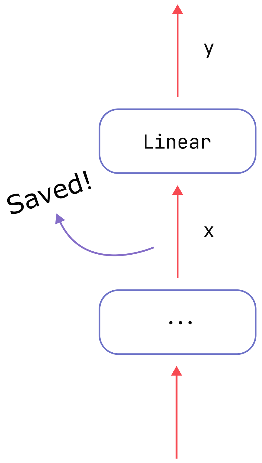
So, as depicted in the figure below, we need to cache the input tensor \(x\) in order to be able to compute the derivative we care about. The cost of saving \(x\) is the source of activation memory for this operation.

In general, in each sub-operation of the type \(y = f(x)\) there may be many intermediate tensors which are created on the way towards generating the output \(y\), and it may not be necessary to save all of them. An efficient implementation of backpropagation (such as torch) will only save any intermediates which are strictly necessary for computing derivatives; any other temporary tensors will be immediately freed. This point will be crucial below: we can compute some activation functions based on their output values alone without needing to cache their inputs.

Case Study: Transformer MLP Layers

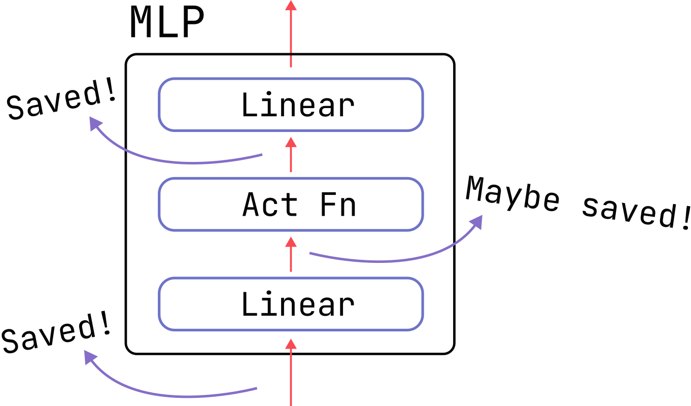
We will use the transformer MLP layers (also known as feed-forward-network or FFN layers) as a testing ground for studying activation memory in detail. A schematic diagram and the corresponding code can be found below.

class MLP(nn.Module):
    """
    Basic MLP (multi-layer perceptron) layer with optional Dropout.
    """

    def __init__(
        self,
        d_model: int,
        act_fn: nn.Module,
        dropout_prob: Optional[float] = None,
        device: Optional[Union[str, torch.device]] = None,
        dtype: Optional[torch.dtype] = None,
    ) -> None:
        super().__init__()
        self.d_model = d_model
        self.act_fn = act_fn
        self.dropout_prob = dropout_prob
        factory_kwargs = {"device": device, "dtype": dtype}

        self.lin_0 = nn.Linear(self.d_model, 4 * self.d_model, **factory_kwargs)
        self.lin_1 = nn.Linear(4 * self.d_model, self.d_model, **factory_kwargs)
        self.dropout = nn.Dropout(self.dropout_prob) if self.dropout_prob else None

    def forward(self, inputs: torch.Tensor) -> torch.Tensor:
        x = self.lin_0(inputs)
        x = self.act_fn(x)
        x = self.lin_1(x)
        if self.dropout is not None:
            x = self.dropout(x)
        return x

Classic Analysis

The activation memory for this block was analyzed in Reducing Activation Recomputation in Large Transformer Models and the result simply comes from adding up the bytes of all the intermediate tensors. Their results are accurate for the GELU case they consider, but we will explain in the following section how changing the activation function can drastically cut activation memory costs.

Here’s a brief recap of their derivation for batch size (b), sequence length (s), and model dimension (d). The sizes of the relevant tensors are:

• (b, s, d) for the inputs to the first Linear layer.
• (b, s, 4 * d) for the inputs to the activation function, because the first linear layer expands the hidden dimension four-fold.
• (b, s, 4 * d) for the inputs to the last linear layer.
• (b, s, d) for the dropout mask, if applicable.

The first three items (which have 9 * b * s * d total elements) have the same dtype as the initial inputs. Assuming the forward pass is performed in lower precision, say torch.bfloat16 which has two bytes per element, the total bytes of activation memory for these tensors is act_mem_mlp = 18 * b * s * d. If Dropout is used, its mask is of type torch.bool whose elements, somewhat confusingly, cost 1 byte (not bit) each and so b * s * d bytes will be added to this result.

Memory-Optimal Activation Functions

While the inputs for GELU need to be saved for backpropagation, this is not true for all activation functions. For some functions, the derivative can be computed entirely from the output values.

For an activation function \(f\) which computes \(y = f(x)\), we need to calculate \(\frac{\partial y}{\partial x}\). The (approximate) GELU function is given by the frightful formula

and the derivative is similarly complex. In this case, there is no way to express \(\frac{\partial y}{\partial x}\) in terms of \(y\) and so we must cache (or recompute) the inputs to get the value of the derivative.

However, for special activations like ReLU and Tanh we do not have to save the inputs because we can write \(\frac{\partial y}{\partial x}\) in terms of \(y\) alone. ReLU is just

and its derivative is extremely simple:

It’s so simple, in fact, that we can equivalently express it in terms of the outputs \(y\):

Tanh also has this property, due to the relation

In general, memory-optimal activation functions have derivatives which can be written in the form \(\frac{d\,y}{dx}= g(y)\) for some function \(g\), meaning they must also be monotonic. They are a special case of autonomous differential equations, as pointed out in this Math Stack Exchange post.

In the transformers MLP layer, we already need to save the outputs of the activation function because they become the inputs to the final Linear layer, and we know from the previous section that these inputs are needed to compute the Linear weight derivatives. So, if we use an activation function which has the special properties above, we can compute activation function derivatives using data we already need to cache anyway and avoid saving the relatively large outputs of the first Linear layer. This represents nearly a factor-of-two savings: the non-dropout activation memory would reduce from 18 * b * s * d to 10 * b * s * d.

Of course, the actual backprop implementation must leverage these special properties in code to realize these gains. Fortunately, torch does, for the most part. The ReLU derivative is defined in these lines derivatives.yaml (which is used to auto-generate code at build time) and is implemented by a simple threshold_backward(grad, result, 0) which enforces the above math and where result is the ReLU output. Compare this with the GELU derivatives defined here which reference self, the input tensor, rather than result.

One activation function which could use reduced memory by default, but which does not in practice (at the time of writing), is LeakyReLU with the default inplace=False setting. This function is

for some number \(s\). If \(s\ge 0\) (as in typical usage), then the derivative can be expressed similarly to the ReLU case

Setting inplace=True in LeakyReLU does realize the expected memory savings, however. (Setting inplace=True in the plain ReLU function is not required.)

Measuring activation memory

The above was theory. Now we turn to code: how to track cached tensors and account for activation memory in torch.

Tensors which are cached during the forward pass can be accessed through the saved_tensors_hooks API, and overall memory readings (on CUDA) can be accessed through torch.cuda.memory_stats. We will use both of these tools in what follows.

Measuring CUDA Memory

torch.cuda.memory_stats contains an incredible amount of information, not all of which is relevant to us. Using this function, we will build a context manager that can be used as follows:

with AllocatedMemContext() as mem:
    loss = Model(inputs)  # Some CUDA computation.

# Memory stats before the computation:
mem.before

# Memory stats after the computation:
mem.after

# Change in memory stats:
mem.delta

In order to illustrate the fields contained by the various dictionaries, consider the following simple example:

with AllocatedMemContext() as mem:
    t1 = torch.randn(2**8, device="cuda")  # 1 KiB
    t2 = torch.randn(2**8, device="cuda")  # 1 KiB
    del t2
    t3 = torch.randn(2**8, device="cuda")  # 1 KiB
    del t3
print(f"{mem.delta=}")

which prints out mem.delta={'allocated': 3072, 'current': 1024, 'freed': 2048, 'peak': 2048}, representing the change in memory usage. These fields mean:

• allocated: newly allocated bytes
• current: bytes used by newly-created and still-alive tensors
• freed: number of bytes freed
• peak: change in peak memory usage

We see that the readings makes sense: above we allocated three tensors t1, t2 of size 1 KiB each (allocated = 3072), with a maximum of two tensors alive at any given moment (peak = 2048). We deleted two of them (freed = 2048), and only one was left surviving (current = 1024). See Zachary Devito’s excellent blog post on the torch CUDA caching allocator for more information about CUDA memory.

WARNING

CUDA libraries are lazily loaded and must be already be on-device to get accurate memory readings. For instance, the first matrix-multiply that is executed will cause ~ 8 MiB of library bytes to be loaded, potentially skewing the results from memory_stats. AllocatedMemContext calls into torch.cuda.current_blas_handle() upon initialization, which ensures that these are loaded before taking readings.

The complete code for the context manager is below:

class AllocatedMemContext:
    def __init__(self) -> None:
        # Ensure CUDA libraries are loaded:
        torch.cuda.current_blas_handle()

        self.before: dict[str, int] = {}
        self.after: dict[str, int] = {}
        self.delta: dict[str, int] = {}

    def _get_mem_dict(self) -> dict[str, int]:
        # Only need `allocated_bytes.all`-prefixed keys here
        key_prefix = "allocated_bytes.all."
        return {
            k.replace(key_prefix, ""): v
            for k, v in torch.cuda.memory_stats().items()
            if key_prefix in k
        }

    def __enter__(self) -> "AllocatedMemContext":
        self.before = self._get_mem_dict()
        return self

    def __exit__(self, *args: Any, **kwargs: Any) -> None:
        self.after = self._get_mem_dict()
        self.delta = {k: v - self.before[k] for k, v in self.after.items()}

Saved Tensors

Now we will build a context manager which will capture the tensors that are saved for use in the backwards pass. The saved_tensors_hooks API will allow us to capture references to all cached tensors.

The API will look like:

model = MyModel(...)
with SavedTensorContext(ignored_tensors=model.parameters()) as saved:
    outputs = model(inputs)

# A dictionary whose keys are the cached tensors
saved.saved_tensors_dict

# The bytes from the cached tensors
saved.saved_tensor_mem

The main subtlety comes in identifying which of these tensors really correspond to separate memory allocations.

To see the issue, consider the weight for some Linear layer, call it lin. We don’t want its weights, lin.weight, to count toward the activation memory costs, since it is already accounted for in the parameter memory budget. But, because the weights are needed in the backward pass, as seen in the matmul example above, the weights will be among the tensors captured by saved_tensors_hooks. We want to exclude the weights’ bytes from saved_tensor_mem (this is what the ignored_tensors argument does), but this is complicated by the fact that the reference will actually be the transposed weight matrix in this case. This means that simple tests like lin.weight is saved_tensor or lin.weight == saved_tensor won’t be able to capture the fact that saved_tensor is really just a view into an object whose memory we are already tracking.

In general, torch will use views wherever possible to avoid new allocations. In the above example, lin.weight and its transpose lin.weight.T correspond to the same chunk of memory and just index into that memory in different ways. As another, example consider splitting a tensor into pieces, as in:

t = torch.randn(16, device="cuda")
split_t = t.split(4)  # A tuple of four tensors

The four tensors in split_t are just views into the original tensor t. The split operation does not cost additional CUDA memory (as can be checked with AllocatedMemContext).

So, how do we tell when two tensors represent slices of the same CUDA memory? PyTorch provides a simple solution: every tensor holds a reference to a Storage class representing the underlying memory, which in turn has a data_ptr method that points to the first element of the tensor’s storage in memory. Two tensors come from the same allocation if their storage’s data_ptrs match. Continuing with the above examples, the following tests pass:

assert all(
    s.untyped_storage().data_ptr() == t.untyped_storage().data_ptr() 
    for s in split_t
)
assert (
    lin.weight.untyped_storage().data_ptr() == lin.weight.T.untyped_storage().data_ptr()
)

WARNING

Tensors also have data_ptr methods themselves, but these return the memory index of the first element that the tensor views into, which is in general different from the first element held by storage. This causes assert all(s.data_ptr() == t.data_ptr() for s in split_t) to fail, for instance.

Here is our context manager which captures references to all tensors saved for the backward pass, but which only counts the memory from distinct allocations:

class SavedTensorContext:
    def __init__(
        self,
        ignored_tensors: Optional[Iterable[torch.Tensor]] = None,
    ) -> None:
        self._ignored_data_ptrs = (
            set()
            if ignored_tensors is None
            else {t.untyped_storage().data_ptr() for t in ignored_tensors}
        )

        self.saved_tensor_dict = torch.utils.weak.WeakTensorKeyDictionary()

        def pack_hook(saved_tensor: torch.Tensor) -> torch.Tensor:
            data_ptr = saved_tensor.untyped_storage().data_ptr()
            if data_ptr not in self._ignored_data_ptrs:
                self.saved_tensor_dict[saved_tensor] = data_ptr
            return saved_tensor

        def unpack_hook(saved_tensor: torch.Tensor) -> torch.Tensor:
            return saved_tensor

        self._saved_tensors_hook = torch.autograd.graph.saved_tensors_hooks(
            pack_hook, unpack_hook
        )

    def __enter__(self) -> "SavedTensorContext":
        self._saved_tensors_hook.__enter__()
        return self

    def __exit__(self, *args: Any, **kwargs: Any) -> None:
        self._saved_tensors_hook.__exit__(*args, **kwargs)

    @property
    def saved_tensor_mem(self) -> int:
        """
        The memory in bytes of all saved tensors, accounting for views into the same storage.
        """
        accounted_for = self._ignored_data_ptrs.copy()
        total_bytes = 0
        for t in self.saved_tensor_dict:
            data_ptr = t.untyped_storage().data_ptr()
            if data_ptr not in accounted_for:
                total_bytes += t.untyped_storage().nbytes()
                accounted_for.add(data_ptr)
        return total_bytes

Example: MLP Block

Let’s use this machinery to confirm our analysis of the MLP block above. Using torch.bfloat16 format (and avoiding mixed-precision for simplicity), we will:

• Loop over the GELU and ReLU versions of the MLP layer.
• Measure the generated CUDA memory and capture the activations.
• Check that the saved activation memory agrees with the measured memory.
• Print out the memory readings and their ratio.

The code:

batch_size, seq_len, d_model = 2, 4096, 1024
dtype = torch.bfloat16
inputs = torch.randn(
    batch_size,
    seq_len,
    d_model,
    device="cuda",
    requires_grad=True,
    dtype=dtype,
)

act_fn_dict = {"ReLU": nn.ReLU(), "GELU": nn.GELU()}
# Append outputs to a list to keep tensors alive
outputs = []
mem_bytes = []

for name, act_fn in act_fn_dict.items():
    mlp = layers.MLP(
        d_model=d_model,
        act_fn=act_fn,
        device="cuda",
        dtype=dtype,
    )
    with act_mem.AllocatedMemContext() as mem, act_mem.SavedTensorContext(
        ignored_tensors=mlp.parameters()
    ) as saved:
        out = mlp(inputs)
        outputs.append(out)
    assert mem.delta["current"] == saved.saved_tensor_mem
    print(f"{name} bytes: {saved.saved_tensor_mem}")
    mem_bytes.append(saved.saved_tensor_mem)

print(f"ReLU/GeLU act mem ratio: {mem_bytes[0]/mem_bytes[1]}")

And the result:

ReLU bytes: 83886080
GELU bytes: 150994944
ReLU/GeLU act mem ratio: 0.5555555555555556

We find perfect agreement with the analysis above: ReLU leverages calculus to cut the memory nearly in half. If we were to peek at the actual tensors in saved.saved_tensor_dict in the two cases, we would see the specific additional tensors which get cached in the GELU case.

Transformer Block Analysis

Lastly, we briefly analyze the savings on the level of the entire transformer block, which includes multi-head attention and residual connections. When using an efficient implementation of the attention mechanism, such as F.scaled_dot_product_attention, the activation memory from the attention block is approximately 10 * b * s * d for torch.bfloat16. The residual connections cost no additional activation memory, because they are simple additions whose derivatives are independent of their inputs.

Working out the numbers, switching out GELU for one of the memory-optimal activation functions at the block level should result in an overall ~25% savings in activation memory. Running the script above with the MLP layers replaced by full transformer Blocks confirms this:

ReLU block bytes: 201523216
GELU block bytes: 268632080
ReLU/GeLU block act mem ratio: 0.7501829863358092

To run the above code yourself, check out the GitHub repo.

A final note: machine learning, like life, is full of trade-offs. Though activation functions like ReLU and Tanh may save a significant amount of memory, GELU is empirically claimed to perform better. What activation function is right for you depends on your specific needs and resources.

Conclusion

In this blog post, we demonstrated how to build simple tools to get insights into the memory usage of torch’s autograd backprop engine, and performed a detailed analysis of the memory advantages of certain activation functions.

There is more that can be done with these tools, e.g they can be used to gain great insight into how torch’s on-the-fly mixed precision autocast works, but we will leave it here for today.