Location via proxy:   [ UP ]  
[Report a bug]   [Manage cookies]                
skip to main content
tutorial
Open access

Graph Time-series Modeling in Deep Learning: A Survey

Published: 28 February 2024 Publication History
  • Get Citation Alerts
  • Abstract

    Time-series and graphs have been extensively studied for their ubiquitous existence in numerous domains. Both topics have been separately explored in the field of deep learning. For time-series modeling, recurrent neural networks or convolutional neural networks model the relations between values across timesteps, while for graph modeling, graph neural networks model the inter-relations between nodes. Recent research in deep learning requires simultaneous modeling for time-series and graphs when both representations are present. For example, both types of modeling are necessary for time-series classification, regression, and anomaly detection in graphs. This article aims to provide a comprehensive summary of these models, which we call graph time-series models. To the best of our knowledge, this is the first survey article that provides a picture of related models from the perspective of deep graph time-series modeling to address a range of time-series tasks, including regression, classification, and anomaly detection. Graph time-series models are split into two categories: (a) graph recurrent/convolutional neural networks and (b) graph attention neural networks. Under each category, we further categorize models based on their properties. Additionally, we compare representative models and discuss how distinctive model characteristics are utilized with respect to various model components and data challenges. Pointers to commonly used datasets and code are included to facilitate access for further research. In the end, we discuss potential directions for future research.

    1 Introduction

    Deep learning research has seen rapid progress in time-series analysis and graph modeling. Time-series analysis is essential in many areas such as signal processing, statistics, and data mining [22, 40, 53]. While there exist many different tasks involving time-series analysis [28, 60], this article specifically focuses on time-series tasks, including time-series classification, time-series anomaly detection, and time-series forecasting. Therefore, we define deep learning models for time-series analysis as a category of models that leverage neural networks to handle time-series data for the aforementioned tasks. Deep learning models for time-series classification typically learn an embedding to classify time-series [48, 87]; Time-series forecasting methods leverage deep learning for various problems such as univariate forecasting [63, 73], multivariate forecasting [8, 82], and forecasting model interpretability [14, 21]; Time-series anomaly detection methods leverage deep learning for anomaly detection at the time-series level [44], at the time-period level [35, 61], and at the time-tick level [18, 98]. Regardless of their specific tasks, these models can be classified into two groups: models that focus on individual time-series and models that simultaneously consider multiple time-series. While the former group typically needs fewer parameters and is easier to interpret, it overlooks the inter-relations between time-series that could potentially enhance model performance. In contrast, models in the latter group either implicitly or explicitly harness the inter-relations between time-series, thereby enabling each time-series to leverage knowledge from others. Graph time-series models, as discussed in this article, exemplify the latter group. Graph models, however, are no less investigated for their universal power to model topological relations between graph node entities [45, 97]. Deep graph learning research has recently seen significant progress in node classification [41, 76], node embeddings [25], and link prediction [94]. In this article, we define graph models as those that leverage a graph structure, where entities of interest are represented as nodes, and their relationships are represented as edges. Graph time-series models fall under the category of graph models, where nodes are associated with time-series.
    Both time-series models and graph models are actively surveyed on their own. Many existing papers survey the topic of either time-series [5, 6, 37] or graphs [97, 102], however, they only enable a partial understanding of models that interweave the two subjects. While a recent paper surveys both topics jointly, it only investigates a specific task of anomaly detection [32]. By contrast, this article aims to fill the gap in available survey papers and provides a timely summary of the joint topic of time-series modeling and graph modeling in deep learning. We refer to related models as deep graph time-series models or graph time-series models for short. Graph time-series models aim to address time-series tasks using two indispensable components, a time-series component that captures the intra-series dependency and a graph component that captures the inter-series dependency. This survey article gives an overview of graph time-series models and provides insights for researchers on what may contribute to model performance.
    In the research area of deep learning, we define graph time-series models as models comprising one or more graphs, where the graph(s) is linked to time-series through their node representations. In a typical graph time-series model, each node of the utilized graph(s) is paired with a time-series. This association extends beyond time-series values and also encompasses the static or dynamic contextual information pertaining to the time-series, if available. Each edge of the graph connects two nodes and indicates the strength of their connection. For instance, in a graph time-series model designed for stock price prediction, a graph can be employed where each node corresponds to the price series and financial status of a company. Edges connecting pairs of stocks potentially indicate the strength of their relationship.
    Our survey is outlined as follows: We compare our article with related survey papers including those that only survey neural time-series models, those that only survey deep graph models, and other related survey papers (Section 2). We provide a high-level picture of how time-series and graphs are modeled on their own in deep learning (Section 3) and then give the preliminary and more technical details on fundamental computations (Section 4). We follow by categorizing representative graph time-series models into two main categories (Section 5), namely, Graph Recurrent/Convolutional Neural Networks (GRCNN) and Graph Attention Neural Networks (GANN). In the GRCNN category, we further categorize models with respect to time-series modeling and graph modeling. In the GANN category, we further categorize models with respect to their targeted tasks. We discuss and analyze the use of representational components in graph time-series models, such as gated mechanism and skip connections, together with the model interpretability (Section 6). Real-world applications and commonly used datasets are summarized; and how graph time-series models adapt to the irregularity, either from time-series or graphs, is also discussed (Section 7). At the same time, we show the performance of selected models on two time-series forecasting tasks to observe what model performs the best and analyze the possible reasons. We include public pointers to datasets and code resources in the appendix (Section D). Open issues and future directions are discussed at the end of the article (Section 8).
    Our article aims to familiarize researchers with state-of-the-art deep graph time-series models. For this purpose, we select and discuss representative papers on the topic. Our key contributions can be summarized as follows:
    To the best of our knowledge, this is the first survey article that unifies the research areas of time-series modeling and graph modeling in deep learning to cover a range of tasks including regression, classification, and anomaly detection. We compile a comprehensive list of related models and detail over 20 representative models.
    To advance the understanding of graph time-series models, we categorize models from various angles, highlight the similarities and differences between models, and have in-depth model discussions.
    We present the performance of selected models on commonly used datasets and give possible reasons on what components contribute to performance improvement.
    We provide insights for future research and application directions in graph-based time-series. Links to publicly used datasets and models are also provided for convenient reference.

    2 Related Survey Papers

    Our survey is closely related to surveys that review either deep time-series models or deep graph models, as well as those review temporal dynamics of graphs from perspectives of temporal point processes or dynamic networks.
    Time-series in deep learning are extensively researched, and many models have been proposed for various tasks. For example, Reference [37] surveys classification models and groups them into generative and discriminative models. Forecasting models [5, 54] are discussed with respect to various task types, such as point forecasting versus probabilistic forecasting, single-horizon forecasting versus multi-horizon forecasting, and so on. Reference [6] provides a taxonomy of anomaly detection models for time-series level, period level, and time-point level outlier detection. Meanwhile, a considerable amount of deep graph models are also studied. For example, Reference [81] provides an overview of representative Graph Neural Networks (GNNs). Another parallel survey paper also summarized different types of GNNs [97]. Moreover, Reference [102] discusses GNNs in terms of different propagation methods, sampling methods, and pooling methods. Although the existing surveys on time-series do not include graph-based models, and the aforementioned surveys on graphs rarely discuss time-series models, these papers and their surveyed models establish a solid foundation for researchers to propose and advance graph time-series models. Recent efforts have aimed at integrating both topics as well. For example, Reference [32] explores graph-based models for time-series anomaly detection. Unlike the exclusive focus on anomaly detection in their work, this article surveys models covering a spectrum of various tasks including regression, classification, and anomaly detection. This serves to bridge the existing gap in the combined domain of time-series modeling and graph modeling in deep learning. The position of our survey scope is illustrated in Figure 1.
    Fig. 1.
    Fig. 1. The scope of our survey article bridges the gap between graph modeling and time-series modeling in deep learning.
    Similar to graph time-series models, temporal point processes in networks and dynamic networks are two types of models that capture the temporal dynamics embedded in a graph structure. Temporal Point Processes (TPP) are random processes that have the realization as a list of discrete events at different time points [23, 42]. TPP is commonly used to model time-series of discrete events in continuous time. For example, TPP-based network models predict the number of link creations in social networks by formulating each link creation as a discrete event, and the time interval between events as a random variable. By contrast, graph time-series models use datasets that aggregate count to derive time-series of a regular time interval. TPP-based models are more refined for temporal modeling, however, they require expert knowledge to select the probabilistic distributions behind random variables, which can be difficult for users without a statistical background. Besides, they typically take quadratic time complexity, which is computationally expensive for large-scale data. Dynamic network models commonly form a time-evolving graph to capture the interactions of nodes for node classification, link prediction, and other tasks [4, 72]. For example, Reference [27] surveys time-dependent graph representation learning and generative modeling. These models do not consider time-series and therefore fail to solve time-series tasks. Different from existing survey papers, this survey primarily addresses two key research questions: RQ1. How do graph time-series models integrate graph models and time-series models, enabling earning the advantages from both? RQ2. How do graph time-series models distinctively incorporate diverse structural designs, such as attention and residual connections? We navigate these research questions throughout the article via in-depth discussion of numerous graph time-series models, which helps readers understand the strength of graph times-series models in tackling various time-series tasks. Moreover, this understanding has the potential to contribute to further advancements within the associated research domain.

    3 Time-series and Graphs in Deep Learning: Individual Modeling

    In this section, we discuss how time-series and graphs are separately modeled in deep learning. Our discussion mainly focuses on the high-level generalization of embedding learning for time-series and nodes in graphs.

    3.1 Time-series Encoding in Deep Learning

    To encode time-series, there are two common types of neural networks: Convolutional Neural Networks (CNNs) and Recurrent Neural Networks (RNNs). Through convolutional filters, CNN models capture local relationships between time-series values within ranges of convolutional filters. RNN models with their recurrent digesting characteristics, instead, aim at learning a hidden state that embeds knowledge from all earlier observations in the time-series, after which the hidden state is used for downstream tasks such as classification or forecasting. Using a multivariate time-series \(\boldsymbol {\mathrm{X}}\in \mathbb {R}^{T \times d}\) of T timesteps and d feature dimensions as an input example, an RNN structure outputs a hidden state \(\mathbf {h}^t \in \mathbb {R}^{d_u}\) for each timestep t of a user-defined \(d_u\) dimensions. A general RNN takes the form
    \(\begin{align} \mathbf {h}^t = f_{\theta }(\mathbf {h}^{t-1}, \mathbf {x}^{t}), \end{align}\)
    (1)
    where \(\theta\) generalizes the structure and parameters of the neural network and \(\mathbf {x}^t \in \mathbb {R}^{d}\) is the observation value vector at timestep t. The starting hidden state \(\mathbf {h}^0\) is typically initialized as \(\boldsymbol {\mathrm{0}}\) when there is no prior knowledge. The model is extended to generalize the case where there are N multivariate time-series as \(X \in \mathbb {R}^{N \times T \times d}\) ; the hidden state \(\boldsymbol {\mathrm{H}}^t \in \mathbb {R}^{N \times d}\) at timestep t is therefore computed by the following equation:
    \(\begin{align} \boldsymbol {\mathrm{H}}^t = f_{\theta }(\boldsymbol {\mathrm{H}}^{t-1}, \boldsymbol {\mathrm{X}}^{t}), \end{align}\)
    (2)
    with \(\boldsymbol {\mathrm{H}}^0\) initialized as \(\boldsymbol {\mathrm{0}}\) and \(\boldsymbol {\mathrm{X}}^t \in \mathbb {R}^{N \times d}\) the observation matrix at timestep t. By having t moving forward along the time dimension, the hidden state at the last timestep \(t=T\) learns from data values at all timesteps. We detail two prevalent RNNs, Long Short-Term Memory (LSTM) and Gated Recurrent Units (GRU), in Section 4.

    3.2 Graph Modeling in Deep Learning

    A great many graph deep learning models have been recently proposed, addressing various graph problems and data natures. In this section, we primarily focus on node embedding models with GNNs. Effective node embeddings can then be used in downstream tasks such as node classification and link prediction.

    3.2.1 Node Embedding.

    Learning informative representations of nodes remains one of the most important tasks in deep graph learning. The learned node embeddings can be used in many tasks [18, 34]. Earlier models leverage random walk [25, 34], while recent models advance node embedding performance with neural network layers that efficiently aggregate neighboring node information and model the non-linear inter-dependency between nodes to assist representation learning [41, 58, 77].
    Given a graph \(G = (V, E)\) with a node set V and an edge set E, and features \(\boldsymbol {\mathrm{X}}\in \mathbb {R}^{N \times d}\) of \(N=|V|\) nodes and d dimensions, the goal of node embedding is to learn a hidden state \(\mathbf {h}_v \in \mathbb {R}^{d_h}\) of a selected dimension \(d_h\) for each node \(v \in V\) . A generalized node embedding graph model takes the form
    \(\begin{align} \mathbf {h}_v = f_{\theta , G} (\boldsymbol {\mathrm{X}}_v, \left\lbrace \mathbf {h}_u \middle | u \in V, u \ne v \right\rbrace), \end{align}\)
    (3)
    where \(\theta\) denotes the GNN structure and parameters. The equation implies that the embedding of node v relies on both its input features and the embeddings of other nodes. In practice, the range of other nodes is limited to a neighborhood set of v, denoted by \(\Gamma (v)\) , thus resulting in \(u \in \Gamma (v)\) .

    3.2.2 Representative Graph Neural Networks.

    GNNs constitute the majority of recent graph-based deep learning models [81, 97]. We briefly introduce how graph structures are leveraged in some of the most successful GNN models.
    Graph Convolutional Networks (GCN) operate directly on graph structures with graph convolutional layers, which is considered a counterpart of CNNs that operate on grid-structured data [41]. For each node in the graph, the GCN model aggregates information from other nodes based on their connection strength, i.e., nodes in proximity have more impact than distant nodes. A graph convolutional layer allows the aggregation of one-hop neighboring nodes. Multi-hop neighborhood aggregation can be achieved by stacking several graph convolutional layers. Essentially, GCN can be seen as a node embedding method and it was initially applied to a node classification task.
    Graph Attention Networks (GAT) integrate the attention mechanism, which consists of self-attentional layers that learn pairwise relations between nodes based on node embeddings [77]. Although the standard GAT takes the graph connectivity information as input, GAT can assume a complete graph when such connectivity information is missing. Node embeddings are used to compute attention scores, which consequently serve as edge weights in the graph. This gives two-fold advantages. First, the attention scores offer a plausibly intuitive interpretation of mutual impacts between nodes. Second, the node embeddings and attention scores can be iteratively computed in turn, providing a self-contained and relatively simple model regarding parameter complexity. Furthermore, external graph structure knowledge, whenever it exists, can be utilized to select attention scores to compute. Similarly, the GAT model can be seen as a node embedding method that learns a hidden state for each node by incorporating their neighborhood information.

    4 Preliminaries and Definitions

    This section defines some symbols and functions for convenience. Additionally, we define commonly used neural modules and formulate time-series tasks. Following typeset conventions are adopted for readability. We use a plain lowercase Latin letter to denote a scalar value or a function (e.g., \(c, d\) as scalar values, \(f(\cdot), g(\cdot)\) as functions), a plain lowercase Greek letter to denote a hyperparameter or a parameter in the neural network (e.g., \(\theta , \psi\) as parameters), a plain uppercase Latin letter to denote a tensor (e.g., \(X\in \mathbb {R}^{N \times T \times d}\) ), a bold lowercase Latin letter to denote a vector (e.g., \(\mathbf {\theta }, \mathbf {b}\) as vectors), a bold uppercase Latin letter to denote a matrix (e.g., \(\boldsymbol {\mathrm{X}}, \boldsymbol {\mathrm{W}}\) as matrices), a calligraphic uppercase Latin letter to denote a set (e.g., \(\mathcal {G} = \lbrace G_1, G_2, \ldots , G_T\rbrace\) ). Subscripts and superscripts are also used to distinguish symbols when they share the same letters. A summary of notations is provided in Table 1. The definitions of time-series, graph, and graph time-series are given as follows:
    Table 1.
    NotationsDescriptionsNotationsDescriptionsNotationsDescriptions
    Xa tensorcnumber of channels \(\boldsymbol {\mathrm{D}}\) degree matrix
    \(\boldsymbol {\mathrm{X}}, \boldsymbol {\mathrm{W}}\) matricesdnumber of features or variates \(\boldsymbol {\mathrm{L}}\) Laplacian matrix
    \(\mathbf {\theta }, \mathbf {a}, \mathbf {b}\) parameter vectors \(\alpha\) attention scoreslnumber of layers
    \(\theta , \psi\) parameter scalar values \(\mathcal {G}\) a series of graphs \(\Vert\) concatenation operator
    Tlength of time-series \(G=(V, E)\) a graph, its node set and edge set \(|\cdot |\) cardinality operator
    wlookback window size \(N =|V|\) number of nodes \(\odot\) Hadamard product
    \(\tau\) future horizon \(\Gamma (v)\) neighbor node set of v \(f_{FC}, f_{EMB}, f_{CONV}\) neural network functions
    \(\mathbf {h}, \boldsymbol {\mathrm{H}}\) hidden states \(\boldsymbol {\mathrm{A}}\) adjacency matrix \(f_{LSTM}, f_{GRU}, g\) neural network modules
    Table 1. A Table Notation of Frequently Used Symbols
    Definition 1 (Time-series).
    A time-series is defined as a sequence of data values either obtained from a continuous space by sampling or recorded in a discrete space. We let \(\mathbf {x}= \left[x_1 x_2 \ldots x_T\right]^\mathsf {T}\in \mathbb {R}^{T}\) containing T observed scalar values denote a univariate time-series of length T. When there are two or more time-series (e.g., d time-series) associated with an entity, a multivariate time-series is usually created and we let \(\boldsymbol {\mathrm{X}}\in \mathbb {R}^{T \times d}\) denote a multivariate time-series of length T and d variates. Some papers use d to denote the number of time features or hidden features. We overload the notation d to denote the number of variates and the number of features, as the context makes it clear which definition is being used. In time-series forecasting tasks, a lookback window containing some most recent values is a common technique to simplify model complexity. We let w denote the window size, and \(\tau\) the prediction horizon.
    Definition 2 (Graph).
    Let \(G = (V, E)\) denote a graph with V and E denoting its node set and edge set. The size of the node set is denoted by \(N = |V|\) , where \(|\cdot |\) denotes the set cardinality operator. The adjacency matrix, denoted by \(\boldsymbol {\mathrm{A}}\in \mathbb {R}^{N \times N}\) , is derived from the edge set, i.e., the element \(A_{ij}\) represents the edge weight from node i to node j. In the case where the graph is a connectivity graph, \(\boldsymbol {\mathrm{A}}\) is instead a binary matrix such that \(\boldsymbol {\mathrm{A}}\in \lbrace 0,1\rbrace ^{N\times N}\) . For each node \(v\in V\) , we let \(\Gamma (v) \subset V\) denote the set of its neighboring nodes. The graph may have node features, in which case, we let \(\boldsymbol {\mathrm{X}}\in \mathbb {R}^{N \times d}\) denote the d dimensional node features. For convenience, we let \(\boldsymbol {\mathrm{L}}, \boldsymbol {\mathrm{D}}\in \mathbb {R}^{N \times N}\) denote the Laplacian matrix and the degree matrix of the adjacency matrix where \(\boldsymbol {\mathrm{L}}= \boldsymbol {\mathrm{D}}- \boldsymbol {\mathrm{A}}\) and \(\boldsymbol {\mathrm{D}}_{ii} = \sum _j \boldsymbol {\mathrm{A}}_{ij}\) .
    Definition 3 (Graph Time-series).
    We define graph time-series as time-series X whose mutual relationships between time-series are described in a graph \(G(V, E, X)\) . Depending on the context, graph time-series can be univariate or multivariate. In graph-based time-series models, each node in the graph is associated with a time-series, hence, there are in total N time-series in the dataset that forms node feature data \(X\in \mathbb {R}^{N \times T \times d}\) of length T and d dimensions. Without loss of generality, the dimension can be set \(d=1\) to include univariate time-series cases. Unless otherwise mentioned, we use a superscript to denote the time index, i.e., \(X^{t}\) denotes all values at the moment t. We use a subscript to denote the node and the multivariate index, i.e., \(X_{i}\) denote all values associated with node i.

    4.1 Fundamental Computations in Neural Networks

    For convenience, we formulate commonly used functions, layers, and modules in neural networks and we let \(f_{*} (\cdot)\) denote them and distinguish them by a subscript, e.g., \(f_{FC}(\cdot)\) stands for a fully connected layer. For the sake of conciseness, activation functions, vectorization, and cornerstone functions such as fully connected layers are depicted in the appendix (Section A). As defined in the appendix, we let \(f_{FC}(\cdot), f_{softmax}(\cdot), f_{EMB}(\cdot), f_{CONV}(\cdot)\) denote a fully connected layer, a softmax layer, an embedding layer, and a convolutional layer, respectively.
    Long Short-Term Memory (LSTM) is one of the most popular RNN variants. The input data to LSTM is a time-series of T timestep and d dimensions, denoted by \(\boldsymbol {\mathrm{X}}\in \mathbb {R}^{T \times d}\) . The time-series is fed to LSTM for each timestep \(t \in \left\lbrace 1, 2, \ldots , T\right\rbrace\) . At any time point t, LSTM digests the input vector \(\boldsymbol {\mathrm{X}}^t \in d\) by the following equations:
    \(\begin{align} \mathbf {f}^t &= \sigma (\boldsymbol {\mathrm{X}}^t \boldsymbol {\mathrm{W}}_{f1} + \mathbf {h}^{t-1} \boldsymbol {\mathrm{W}}_{f2} + \mathbf {b}_f) &\quad \mathbf {i}^t &= \sigma (\boldsymbol {\mathrm{X}}^t \boldsymbol {\mathrm{W}}_{i1} + \mathbf {h}^{t-1} \boldsymbol {\mathrm{W}}_{i2} + \mathbf {b}_i) \end{align}\)
    (4)
    \(\begin{align} \mathbf {o}^t &= \sigma (\boldsymbol {\mathrm{X}}^t \boldsymbol {\mathrm{W}}_{o1} + \mathbf {h}^{t-1} \boldsymbol {\mathrm{W}}_{o2} + \mathbf {b}_o) &\quad \mathbf {c}^t &= \mathbf {f}^t \odot \mathbf {c}^{t-1} + vi^t \odot \tanh (\boldsymbol {\mathrm{X}}^t \boldsymbol {\mathrm{W}}_{c1} + \mathbf {h}^{t-1} \boldsymbol {\mathrm{W}}_{c2} + \mathbf {b}_c) \end{align}\)
    (5)
    \(\begin{align} \mathbf {h}^t &= \mathbf {o}^t \odot \mathbf {c}^t , \end{align}\)
    (6)
    where \(\odot\) denotes the Hadamard product. The dimension \(c_{in} = d\) is transformed to the dimension \(c_{out}\) . The dimensions of the variables are \(\mathbf {f}^t, \mathbf {i}^t, \mathbf {o}^t, \mathbf {c}^t, \mathbf {h}^t \in \mathbb {R}^{c_{out}}\) , \(\boldsymbol {\mathrm{W}}_{*1} \in \mathbb {R}^{c_{in} \times c_{out}}\) , \(\boldsymbol {\mathrm{W}}_{*2} \in \mathbb {R}^{c_{out} \times c_{out}}\) , and \(\mathbf {b}_* \in \mathbb {R}^{c_{out}}\) . Variables \(\mathbf {f}^0, \mathbf {i}^0, \mathbf {o}^0, \mathbf {c}^0, \mathbf {h}^0\) are initialized with user-selected values (e.g., \(\mathbf {0}\) ). Thus, we let \(f_{LSTM} (\boldsymbol {\mathrm{X}}) = [h^1 h^2 \cdots h^T]^\mathsf {T}\in \mathbb {R}^{T \times c_{out}}\) denote LSTM.
    Gated Recurrent Units (GRU) is another popular RNN variant. With the same input \(\boldsymbol {\mathrm{X}}\in \mathbb {R}^{T \times d}\) as that to LSTM, GRU is described by the following equations:
    \(\begin{align} \mathbf {r}^t &= \sigma \left(\boldsymbol {\mathrm{X}}^t \boldsymbol {\mathrm{W}}_{r1} + \mathbf {h}^{t-1}\boldsymbol {\mathrm{W}}_{r2} + \mathbf {b}_r \right) &\quad \mathbf {u}^t &= \sigma \left(\boldsymbol {\mathrm{X}}^t \boldsymbol {\mathrm{W}}_{u1} + \mathbf {h}^{t-1}\boldsymbol {\mathrm{W}}_{u2} + \mathbf {b}_u\right) \end{align}\)
    (7)
    \(\begin{align} \mathbf {c}^t &= \tanh \left(\boldsymbol {\mathrm{X}}^t \boldsymbol {\mathrm{W}}_1 + \left(\mathbf {r}^t \odot \mathbf {h}^{t-1}\right) \boldsymbol {\mathrm{W}}_2 + \mathbf {b}\right) &\quad \mathbf {h}^t &= \mathbf {u}^t \odot \mathbf {h}^{t-1} + \left(1-\mathbf {u}^t\right) \odot \mathbf {c}^t , \end{align}\)
    (8)
    where the dimensions of variables are \(\mathbf {r}^t, \mathbf {u}^t, \mathbf {c}^t, \mathbf {h}^t \in \mathbb {R}^{c_{out}}\) , \(\boldsymbol {\mathrm{W}}_{*1} \in \mathbb {R}^{c_{in} \times c_{out}}\) , \(\boldsymbol {\mathrm{W}}_{*2} \in \mathbb {R}^{c_{out} \times c_{out}}\) , and \(\mathbf {b}_* \in \mathbb {R}^{c_{out}}\) . Thus, we let \(f_{GRU} (\boldsymbol {\mathrm{X}}) = [ h^1 h^2 \cdots h^T ]^\mathsf {T}\in \mathbb {R}^{T \times c_{out}}\) denote the GRU module function.
    Graph Convolutional Neural Network (GCN) is a fundamental GNN model that transforms node features with a graph structure. Given a graph \(G=(V, E, \boldsymbol {\mathrm{A}})\) and node features \(\boldsymbol {\mathrm{X}}\in \mathbb {R}^{N \times d}\) , a GCN model with l graph convolutional layers learns node embeddings by
    \(\begin{align} \hat{\boldsymbol {\mathrm{A}}} &= \boldsymbol {\mathrm{A}}+ \boldsymbol {\mathrm{I}}&\ \ \hat{\boldsymbol {\mathrm{D}}}_{ii} &= \sum _j \hat{\boldsymbol {\mathrm{A}}}_{ij} &\ \ \tilde{\boldsymbol {\mathrm{A}}} &= \hat{\boldsymbol {\mathrm{D}}}^{-\frac{1}{2}} \hat{\boldsymbol {\mathrm{A}}} \hat{\boldsymbol {\mathrm{D}}}^{-\frac{1}{2}} &\ \ \boldsymbol {\mathrm{H}}^0 &= \boldsymbol {\mathrm{X}}&\ \ \boldsymbol {\mathrm{H}}^l &= f_{GCN}^{l}(X, \boldsymbol {\mathrm{A}}) = \sigma (\tilde{\boldsymbol {\mathrm{A}}} \boldsymbol {\mathrm{H}}^{l-1} \boldsymbol {\mathrm{W}}^{l-1}), \end{align}\)
    (9)
    where \(\boldsymbol {\mathrm{A}}, \boldsymbol {\mathrm{I}}, \boldsymbol {\mathrm{D}}, \hat{\boldsymbol {\mathrm{A}}}, \hat{\boldsymbol {\mathrm{D}}} \in \mathbb {R}^{N \times N}\) are adjacency matrix, identity matrix, diagonal matrix, normalized adjacency matrix, and normalized degree matrix, respectively. \(\boldsymbol {\mathrm{W}}^* \in \mathbb {R}^{c_{in,*} \times c_{out,*}}\) where \(c_{in,0} = d\) , and \(c_{in,l} = c_{out,l-1}\) . When the context is clear, we let \(f_{GCN} (X)\) denote \(f_{GCN} (X, \boldsymbol {\mathrm{A}})\) .
    Graph Attention Network (GAT) is another powerful GNN. GAT relies on attention scores instead of explicit edge weights for node message aggregation. The attention coefficients are computed with:
    \(\begin{align} \alpha _{ij} &= \frac{\exp \left(\text{LeakyReLU}\left(\mathbf {a}^\mathsf {T}\left[\boldsymbol {\mathrm{W}}\boldsymbol {\mathrm{H}}_i \Vert \boldsymbol {\mathrm{W}}\boldsymbol {\mathrm{H}}_j \right]\right)\right)}{\sum _{k\in \Gamma _i \cup \left\lbrace i\right\rbrace } \exp \left(\text{LeakyReLU}\left(\mathbf {a}^\mathsf {T}\left[\boldsymbol {\mathrm{W}}\boldsymbol {\mathrm{H}}_i \Vert \boldsymbol {\mathrm{W}}\boldsymbol {\mathrm{H}}_k \right]\right)\right)} \end{align}\)
    (10)
    \(\begin{align} \boldsymbol {\mathrm{H}}_i^{\prime } &= \sigma \left(\frac{1}{K} \sum _{k=1}^K \sum _{j\in \Gamma _i \cup \lbrace i\rbrace } \alpha _{ij}^k \boldsymbol {\mathrm{W}}^k \boldsymbol {\mathrm{H}}_j\right) , \end{align}\)
    (11)
    where \(\alpha _{ij}\) is the attention score from node j in the neighboring node set \(\Gamma _i\) to node i, which is calculated by obtaining scores for all neighboring nodes of i, with a trainable parameter matrix \(\boldsymbol {\mathrm{W}}\) and concatenated hidden states (denoted by concatenation operator \(\Vert\) ) \(\boldsymbol {\mathrm{H}}_i\) and \(\boldsymbol {\mathrm{H}}_j\) of node i and j. A neural network layer \(\text{LeakyReLU}\left(\mathbf {a}^\mathsf {T}(\cdot)\right)\) is applied with a trainable parameter vector \(\mathbf {a}\) and a softmax normalization, as described by Equation (10).
    The attention scores can be extended to K channels, therefore, a new hidden state \(\boldsymbol {\mathrm{H}}_i^{\prime }\) for node i is calculated as the average of multi-head attention, and each channel is calculated with attention scores \(\mathbf {a}_{ij}^{k}\) , the trainable parameter matrix \(\boldsymbol {\mathrm{W}}^k\) , and hidden states in the local neighborhood \(\boldsymbol {\mathrm{H}}_j\) where \(j\in {\Gamma _i \cup \lbrace i\rbrace }\) , of node i.

    4.2 Problem Definitions

    Graph time-series models essentially target various time-series tasks; this section formulates some of the most important ones, namely, time-series classification [46, 64, 65, 92], time-series forecasting [8, 12, 47, 57, 62, 67, 70, 75, 79, 84], and anomaly detection on time-series [7, 18, 98]. Without the loss of generality, we assume the input to all these tasks are multiple multivariate time-series X and a graph G. Each time-series is associated with a node in G.
    Graph Time-series Classification aims to predict labels of time-series. Assuming the input is time-series \(\boldsymbol {\mathrm{X}}\in \mathbb {R}^{N \times T \times d}\) and there is a label set \(\mathcal {Y}= \left\lbrace 1, 2, \ldots , C\right\rbrace\) of C different classes, a classification model learns a mapping from each time-series to its label \(f_{\text{classification}}: \left(G, X\right) \mapsto \mathbf {y}\) where \(\mathbf {y}\in \mathcal {Y}^{N}\) .
    Graph Time-series Forecasting aims to predict values in the future horizon given historical observations. Assuming the input is time-series \(\boldsymbol {\mathrm{X}}\in \mathbb {R}^{N \times T \times d}\) and the target prediction horizon is \(\tau\) , a forecasting model learns a mapping from the time-series to predicted future values \(f_{\text{forecasting}}: \left(G, X^{1:T}\right) \mapsto \hat{X}^{T+1:T+\tau }\) .
    Graph Time-series Anomaly Detection can be categorized into three levels, N.e., time-series level, period level, and time point level. Time-series level anomaly detection tasks are essentially binary classification tasks where a time-series is classified as normal or not normal. Period-level anomaly detection aims to find out irregular periods of the time-series. Given time-series \(\boldsymbol {\mathrm{X}}\in \mathbb {R}^{N \times T}\) , a period-level anomaly detection model learns a mapping from the time-series to a set of periods \(f_{detection}: \boldsymbol {\mathrm{X}}\mapsto \left\lbrace (s_p, t_p) | p = 1, 2, \ldots , P\right\rbrace\) , where P is the number of detected anomalous periods. Time point level anomaly detection can be seen as a special case of the period level where the period has a length of 1. These fundamental definitions can be modified without difficulty to agree with the actual formulation such as dynamic graphs or multivariate time-series.

    5 Deep Graph Time-series Modeling

    Recent graph time-series models are primarily divided into two categories: Graph Recurrent/Convolutional Neural Networks (GRCNN) and Graph Attention Neural Networks (GANN). GRCNN models leverage autoregressive or convolutional layers to learn the temporal dependency between time values (Section 5.1.1 and Section 5.1.2). We also discuss GRCNN models regarding the use of self-derived graphs (Section 5.1.3) and evolving graphs (Section 5.1.4). GANN models integrate attention mechanisms to capture the dependency. Different attention mechanisms provide possible interpretations of mutual impact between nodes and between values across timestamps. We discuss the different attention types in detail throughout Section 5.2. Note that our categories are not exclusive, and a model may fall into different categories. In this situation, we discuss the model in the most appropriate category. Throughout the discussion, we summarize and highlight the key functions or modules of the introduced models, with detailed model equations included in the appendix (Section B) for reference. A timeline of surveyed models is provided in Table 2. Pointers to related experimental setups such as time-series normalization and graph construction and available code resources are also given in the appendix (Section C and Section D).
    Table 2.
    YearsGraph Recurrent/Convolutional Neural NetworksGraph Attention Neural Networks
    2018 or beforeGCRN [69], DCRNN [51], STGCN [90]GaAN [92]
    2019Graph WaveNet [83], T-GCN [100], LRGCN [46]ASTGCN [26]
    2020MTGNN [82], DGSL [70]MTAD-GAT [98], STAG-GCN [57]
    STGNN [79], Cola-GNN [19], ST-GRAT [66]
    2021FC-GAGA [62], Radflow [75]GDN [18], StemGNN [8]
    STFGNN [47], Z-GCNET [12], TStream [11]
    2022VGCRN [10], GRIN [13], RGSL [91], GANF [16]GReLeN [95], FuSAGNet [29], THGNN [85]
    ESG [88] 
    Table 2. Representative Graph Time-series Models

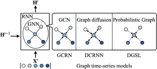
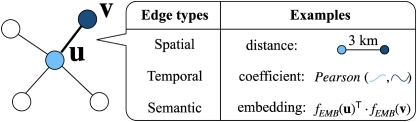
    5.1 Graph Recurrent/Convolutional Neural Networks

    An intuitive way of modeling graphs and time-series is to combine a graph model and a time-series model. In deep learning, RNN and CNN are commonly used for the time-series model, while GNN is used for the graph model. Table 3 provides a comparison of GRCNN with respect to their time-series modeling and graph modeling. Most GRCNN models build a graph where each node is associated with a time-series, either univariate or multivariate. Unless otherwise mentioned and without loss of generality, we assume the associated time-series are all multivariate and share the same feature dimension size in all nodes. In this section, we first discuss models from the perspective of time-series modeling, as in Section 5.1.1 and Section 5.1.2, then we discuss models from the perspective of graph modeling, as in Section 5.1.3 and Section 5.1.4. We summarize the model attributes in Table 3.
    Table 3.
    CategoriesModelsTime-seriesPropagationGraph TypesEvolving Graphs
    RNNCNNGatesGCNDiffusionGatesSpatialTemporalSemantic
    RNN-based Graph Time-series Modeling (Section 5.1.1)GCRN [69] \(\checkmark\)    \(\checkmark\)    \(\checkmark\)    
    DCRNN [51] \(\checkmark\)     \(\checkmark\)   \(\checkmark\)    
    T-GCN [100] \(\checkmark\)    \(\checkmark\)    \(\checkmark\)    
    DGSL [70] \(\checkmark\)     \(\checkmark\)     \(\checkmark\)  
    VGCRN [10] \(\checkmark\)    \(\checkmark\)      \(\checkmark\)  
    GANF [16] \(\checkmark\)    \(\checkmark\)    \(\checkmark\)    
    GRIN [13] \(\checkmark\)    \(\checkmark\)    \(\checkmark\)    
    CNN-based Graph Time-series Modeling (Section 5.1.2)STGCN [90]  \(\checkmark\)   \(\checkmark\) \(\checkmark\)      
    G-WaveNet [83]  \(\checkmark\)   \(\checkmark\)    \(\checkmark\)   \(\checkmark\)  
    MTGNN [82]  \(\checkmark\)   \(\checkmark\)     \(\checkmark\)   
    Models with Self-derived Graphs (Section 5.1.3)FC-GAGA [62]   \(\checkmark\)    \(\checkmark\)   \(\checkmark\) \(\checkmark\)  
    STFGNN [47] \(\checkmark\)     \(\checkmark\)   \(\checkmark\) \(\checkmark\)   
    RGSL [91] \(\checkmark\)    \(\checkmark\)    \(\checkmark\)   \(\checkmark\)  
    Models with Evolving Graphs (Section 5.1.4)Radflow [75] \(\checkmark\)       \(\checkmark\)    \(\checkmark\)
    TStream [11] \(\checkmark\)    \(\checkmark\)    \(\checkmark\)    \(\checkmark\)
    LRGCN [46] \(\checkmark\)    \(\checkmark\)    \(\checkmark\)    \(\checkmark\)
    Z-GCNET [12]  \(\checkmark\)   \(\checkmark\)    \(\checkmark\)    \(\checkmark\)
    ESG [88] \(\checkmark\)   \(\checkmark\) \(\checkmark\)    \(\checkmark\) \(\checkmark\)   \(\checkmark\)
    Table 3. An Attribute Comparison of GRCNN Models

    5.1.1 RNN-based Time-series Modeling.

    RNN models, as described in Equation (4)–Equation (8), can perform node message propagation by substituting the weight matrix multiplication with graph convolution or graph diffusion. Hence, the modified RNN models not only model the temporal dependency through its recursive nature but also capture the non-linear mutual impacts among nodes. In this category, we cover GCRN, DCRNN, and DGSL, all of which nest the GNN model within an RNN cell, as depicted in Figure 2.
    Fig. 2.
    Fig. 2. A diagram of Graph RNN models. The graph component (e.g., GCN or diffusion) is nested within the RNN cells.
    GCRN [69] substitutes fully connected layers in LSTM with graph convolutional layers. Specifically, the weight matrix multiplication for all gates in the LSTM is replaced with GCN, resulting in an LSTM variant denoted as \(\text{LSTM}^\ast\) ,
    \(\begin{align} \boldsymbol {\mathrm{H}}^t = \text{LSTM}^\ast _{f_{GCN}, G} (\boldsymbol {\mathrm{X}}^t, \boldsymbol {\mathrm{H}}^{t-1}). \end{align}\)
    (12)
    GCRN leverages the graph structure for training, which allows each node to efficiently aggregate neighborhood information, in contrast to a raw RNN (in this case, the LSTM model) that models the dependency between nodes by dense neural layers. The GCRN model takes a similar form to an LSTM model, therefore, the derived hidden state in Equation (46) is sensibly used in time-series forecasting tasks in the same way as how the hidden state is used in LSTM. See Section B.1 for detailed equations.
    DCRNN [51] uses diffusion convolution to replace the weight matrix multiplication in a different RNN variant, the Gated Recurrent Units (GRU). The graph diffusion operator, denoted by \(g_\mathbf {\theta }(\cdot)\) with respect to parameters \(\mathbf {\theta }\) and an adjacency matrix \(\boldsymbol {\mathrm{A}}\) , is defined as
    \(\begin{align} g_\mathbf {\theta }(\boldsymbol {\mathrm{X}}) = \sum _{k=0}^{K-1} \left(\theta _{k, 1} (\boldsymbol {\mathrm{D}}_O^{-1} \boldsymbol {\mathrm{A}})^k + \theta _{k, 2} (\boldsymbol {\mathrm{D}}_I^{-1} \boldsymbol {\mathrm{A}}^\mathsf {T})^k \right)\boldsymbol {\mathrm{X}}, \end{align}\)
    (13)
    where \(\boldsymbol {\mathrm{D}}_O, \boldsymbol {\mathrm{D}}_I\) denotes the in-degree matrix and the out-degree matrix, respectively. The model utilizes the random walk matrix \(\boldsymbol {\mathrm{D}}_O^{-1} \boldsymbol {\mathrm{A}}\) and \(\boldsymbol {\mathrm{D}}_I^{-1} \boldsymbol {\mathrm{A}}^\mathsf {T}\) for information propagation. Regarding the temporal component, GRU is chosen instead of LSTM, which brings the benefit of lighter computing workloads due to the simpler structure of GRU model. DCRNN inspires many subsequent models, including DGSL [70], T-GCN [100], and GraphDF [9].
    DGSL [70] can be seen as a DCRNN variant with a probabilistic graph, where the graph structure is learned from time-series data. Given time-series data \(X \in \mathbb {R}^{N \times T \times d}\) , a graph \(\boldsymbol {\mathrm{A}}\in \left\lbrace 0, 1 \right\rbrace ^{N\times N}\) is parameterized and sampled by the following equations:
    \(\begin{align} \boldsymbol {\mathrm{Z}}_i &= f_{FC, z} \left(\text{Vec}\left(f_{conv, T} (\boldsymbol {\mathrm{X}}_i) \right) \right) &\quad \theta _{ij} &= \sigma \left(f_{FCs} \left(\boldsymbol {\mathrm{Z}}_i \Vert \boldsymbol {\mathrm{Z}}_j \right) \right) \end{align}\)
    (14)
    \(\begin{align} \boldsymbol {\mathrm{A}}_{ij} &= \sigma \left(\frac{\log \frac{\theta _{ij}}{1-\theta _{ij}} + \left(g_{ij}^1 - g_{ij}^2\right)}{s} \right) ,\quad i,j \in \lbrace 1, 2, \ldots , N\rbrace , \end{align}\)
    (15)
    where \(g_{ij}^1, g_{ij}^2 \sim \text{Gumbel}(0, 1)\) (Defined in Section C.5). A binary graph is constructed by sampling edges from distributions in Equation (15), which leverages the Gumbel reparameterization method [38], with s a selected constant parameter. The parameter \(\theta _{ij}\) for each node pair is learned from a link prediction method that takes node embeddings as input as in Equation (14). With the sampled graph, DGSL renders the DCRNN model for sequence-to-sequence training and forecasting. Since the graph in DGSL is parameterized with the time-series data, it optimizes trainable parameters for both time-series and graph learning simultaneously.
    More recent methods construct graphs in various ways for tasks other than time-series forecasting. For instance, VGCRN [10] takes a probabilistic approach and builds a deep variational network for time-series anomaly detection. GANF [16] builds a graph-augmented flow model with a Bayesian network that models the causal relationships between time-series for time-series anomaly detection. Moreover, GRIN [13] targets time-series imputation with GNN and RNN.
    Model Comparison. For graph modeling, GCRN uses GCN that operates on undirected graphs, while DCRNN and DGSL use graph diffusion, which has the advantage of modeling directed graphs. Further, GCRN and DCRNN require external graph structures, while DGSL takes a probabilistic approach and learns graph structures from node embeddings without using a pre-defined graph. A diagram of Graph RNN cell is shown in Figure 3, which highlights the distinctions and commonalities among the chosen models.
    Fig. 3.
    Fig. 3. A detailed diagram of a Graph RNN cell. \(\boldsymbol {\mathrm{X}}^t\) denotes values from different time-series at time t. Each node is associated with an individual time-series. The inter-relations between time-series are captured through GNN, which is differently employed among the selected graph time-series models. In GCRN, each node learns from its neighbors through GCN. In DCRNN, its diffusion learning process considers both the in-degree and out-degree of each node, as represented by the dual-headed arrows. In DGSL, the utilized graph structure is probabilistic, as indicated by the dashed arrows.

    5.1.2 CNN-based Time-series Modeling.

    Another line of work models time-series through CNN instead of RNN.
    STGCN [90] models the graph structure and temporal dependence individually with separate layers, instead of nesting graphs in the RNN structure. STGCN proposes a spatio-temporal convolutional block that consists of temporal-spatial-temporal layers. The temporal layer is built upon a 1D convolutional layer with gated linear units and requires less time complexity compared to RNN models. The spatial layer, however, is made of a GCN layer. Therefore, STGCN inspires a separate and individual view and usage of temporal and spatial dimensions.
    Graph WaveNet [83] points out that the explicitly given graph structure may not be able to represent relations between nodes due to missing node connections. To mitigate the missing information and the ineffectiveness of the RNN component, Graph WaveNet develops an adaptive adjacency matrix and it also replaces RNN models with stacked dilated convolutional layers. With respect to the graph modeling, Graph WaveNet adapts the graph diffusion layer from DCRNN by adding a third term of an adaptive adjacency \(\boldsymbol {\mathrm{A}}_{adapt}\) to the diffusion matrix in Equation (13):
    \(\begin{align} \boldsymbol {\mathrm{A}}_{adapt} = f_{softmax} \left(\text{ReLU}\left(\boldsymbol {\mathrm{H}}_{emb1} \boldsymbol {\mathrm{H}}_{emb2}^\mathsf {T}\right) \right), \end{align}\)
    (16)
    where the adaptive matrix is learned through the embeddings \(\boldsymbol {\mathrm{H}}_{emb1}\) and \(\boldsymbol {\mathrm{H}}_{emb2}\) , which are independent of the given graph structure. Both \(\boldsymbol {\mathrm{H}}_{emb1}\) and \(\boldsymbol {\mathrm{H}}_{emb2}\) are randomly initialized in the beginning of model training.
    MTGNN [82] also builds a graph through node embeddings and requires no prior graph structure knowledge. MTGNN models time-series and graphs separately and subsequently incorporates them in a pipeline order. For the sake of conciseness, we focus on the graph modeling part and let \(g_{cnn} (\cdot)\) denote the temporal component, which renders dilated CNN layers to drastically reduce the temporal dimension of time-series. Given time-series data \(\boldsymbol {\mathrm{X}}\in \mathbb {R}^{N \times T \times D}\) , node embeddings \(\boldsymbol {\mathrm{H}}_{{emb}_1}, \boldsymbol {\mathrm{H}}_{{emb}_2} \in \mathbb {R}^{N \times d_{emb}}\) , the adjacency matrix is computed by
    \(\begin{align} \boldsymbol {\mathrm{Z}}_1 &= \tanh \left(\alpha f_{FC, W_1} \left(\boldsymbol {\mathrm{H}}_{{emb}_1}\right) \right) &\quad \boldsymbol {\mathrm{Z}}_2 &= \tanh \left(\alpha f_{FC, W_2} \left(\boldsymbol {\mathrm{H}}_{{emb}_2}\right) \right), \end{align}\)
    (17)
    \(\begin{align} \boldsymbol {\mathrm{A}}_0 &= \text{ReLU}\left(\tanh \left(\alpha \left(\boldsymbol {\mathrm{Z}}_1 \boldsymbol {\mathrm{Z}}_2^\mathsf {T}- \boldsymbol {\mathrm{Z}}_2 \boldsymbol {\mathrm{Z}}_1^\mathsf {T}\right)\right)\right) &\quad \boldsymbol {\mathrm{A}}&= \text{topk}_{row} (\boldsymbol {\mathrm{A}}_0), \end{align}\)
    (18)
    where two individually calculated node embeddings are transformed by dense layers and a \(\tanh (\cdot)\) activation together with a selected constant hyperparameter \(\alpha\) , as shown in Equation (17). Note that \(\boldsymbol {\mathrm{A}}\) is ensured to be asymmetric, and row-wise top K selections are used to further sparsify connections, as formulated in Equation (18).
    To preserve the initial graph structure denoted by \(\boldsymbol {\mathrm{A}}\) , MTGNN leverages a random walk with restart method to derive multi-level hidden states for each node and thereafter concatenates all hidden states. Let \(\boldsymbol {\mathrm{H}}^0 = g_{cnn} \left(\boldsymbol {\mathrm{X}}\right)\) denote the initial hidden state from the temporal component, the multi-level hidden states are computed and aggregated with the transformed graph structure \(\tilde{\boldsymbol {\mathrm{A}}}\) from Equation (9), resulting in the hidden states at l layer as
    \(\begin{align} \boldsymbol {\mathrm{H}}^l &= \beta \boldsymbol {\mathrm{H}}^0 + (1-\beta) \tilde{\boldsymbol {\mathrm{A}}} \boldsymbol {\mathrm{H}}^{l-1}, \end{align}\)
    (19)
    \(\begin{align} \boldsymbol {\mathrm{H}}&= \sum _l f_{FC, W_l} (\boldsymbol {\mathrm{H}}^l). \end{align}\)
    (20)
    Model Comparison. STGCN, Graph WaveNet, and MTGNN use different CNN variants for time-series modeling. STGCN uses gated causal CNN and Graph WaveNet uses dilated CNN. MTGNN combines several dilated CNNs to derive the inception dilated CNN, which allows it to model time-series values regarding various granularities. We also notice that STGCN uses a GCN layer to model the provided spatial graph, while Graph WaveNet proposes an adaptive graph that combines both the spatial graph and the self-derived semantic graph. MTGNN only relies on a self-derived semantic graph and requires no provided graph in the datasets. Model Comparison on Time-series Components: RNN versus CNN. To model a time-series in deep learning, one of the most intuitive ways is to apply a fully connected layer or a series of fully connected layers on the input time-series data and update network parameters by fitting predicted values with actual ground truth [5]. Each neuron in the input layer holds a value for each timestep, and neurons in the following layer summarize values at all timesteps by network parameters, however, this leads to an explosive growth of parameters and inefficiency of optimization as the number of layers increases. To address these issues, convolutional layers are more often used, which drastically reduce model complexity with fewer neural connections between layers. Further, a dilated CNN layer (shown in Figure 4) models very long sequences with low model complexity, as it down-samples the time-series input with a pre-selected frequency. CNN-based models are also called direct methods, since they predict future values in one shot [19]; on the contrary, RNN-based models capture the temporal dependency by recurrently consuming the time values to derive a final embedding. Due to this time-series modeling nature, RNN is most widely used in temporal modeling, as we expound on it in Section 3.1. RNN-based graph time-series models nest the graph modeling within the RNN cells and are therefore relatively more constrained regarding the model design, compared to CNN-based models where graph and time-series are separately modeled with different layers, which allows diverse combinations such as the temporal-spatial-temporal structure in STGCN.
    Fig. 4.
    Fig. 4. A model with three dilated CNN layers (dilation factor as \(\left[1, 2, 4\right]\) ) can digest 8 time values, which is typically faster than an RNN structure unfolding 8 times.

    5.1.3 Models with Self-derived Graphs.

    Most related datasets such as traffic data and electricity workload data provide an external graph that primarily describes the geographical connectivity of nodes, however, external graph structures are not always available, and they do not necessarily reflect the actual connections between nodes. In these situations, several models propose using self-derived graphs, i.e., the graph structure is derived either from time-series or from node embeddings. This section describes models from the perspective of graph modeling, specifically, on how different models leverage self-derived graphs to capture the inter-relations between nodes. We discuss three models in this section: FC-GAGA [62], STFGNN [47], and RGSL [91], but other models such as Graph WaveNet and MTGNN, which are discussed in the previous section, also belong to this category. The graph types in different models are summarized in Table 3. At the end of this section, we compare models in terms of their graph modeling.
    FC-GAGA [62], similar to MTGNN, requires no prior knowledge of the graph structure. Note that FC-GAGA uses time-series gates instead of RNN or CNN for time-series modeling. The time-series gates can be seen as a special type of CNN, as they are used to weight time co-variate features. Let \(\boldsymbol {\mathrm{X}}\in \mathbb {R}^{N \times T}\) denote the node time-series, and let \(\boldsymbol {\mathrm{H}}_{emb}=f_{EMB}\left(\boldsymbol {\mathrm{X}}\right) \in \mathbb {R}^{N \times d_{emb}}\) denote the node embeddings. FC-GAGA is described by the following equations:
    \(\begin{align} \boldsymbol {\mathrm{A}}&= \exp (\epsilon \boldsymbol {\mathrm{H}}_{emb} \boldsymbol {\mathrm{H}}_{emb} ^\mathsf {T}) &\quad \tilde{\mathbf {x}}_i &= \max _j \boldsymbol {\mathrm{X}}_{ij} &\quad \boldsymbol {\mathrm{G}}_{i,jk} &= \text{ReLU}{\left[ \frac{\boldsymbol {\mathrm{A}}_{ij} \boldsymbol {\mathrm{X}}_{jk} - \tilde{\mathbf {x}}_i}{\tilde{\mathbf {x}}_i} \right]} , \end{align}\)
    (21)
    \(\begin{align} \boldsymbol {\mathrm{Z}}&= \left[\boldsymbol {\mathrm{H}}_{emb} \Vert \frac{\boldsymbol {\mathrm{X}}}{\tilde{\mathbf {x}}} \Vert \boldsymbol {\mathrm{G}}\right]^\mathsf {T}&\quad \hat{\boldsymbol {\mathrm{X}}} &= f_{res} \left(\boldsymbol {\mathrm{Z}}\right) , \end{align}\)
    (22)
    where the graph structure \(\boldsymbol {\mathrm{A}}\) is learned and optimized from the node embeddings and is used together with transformed time-series data \(\tilde{\mathbf {x}}_i\) in a gated mechanism to shut off connections of irrelevant node pairs as in Equation (21), with \(\epsilon\) as a selected constant hyperparameter. A hidden state \(\boldsymbol {\mathrm{Z}}\) is constructed from a concatenation of node embedding \(\boldsymbol {\mathrm{H}}_{emb}\) , scaled time-series data \(\boldsymbol {\mathrm{X}}/ \tilde{\mathbf {x}}\) , and the gated states \(\boldsymbol {\mathrm{G}}\) . Subsequently, \(\boldsymbol {\mathrm{Z}}\) serves as the initial input for a residual module, denoted by \(f_{res}\) , which generates the time-series prediction \(\hat{\boldsymbol {\mathrm{X}}}\) . For the purpose of conciseness, we include the details of the residual module \(f_{res}\) in Section B.2. FC-GAGA benefits from the freedom of automatically deriving graph structures, instead of relying on the Markov model-based or distance-based graph topological information. However, the graph construction from node embedding costs a time complexity of \(\mathcal {O}\left(N^2\right)\) , which limits the scalability of FC-GAGA.
    STFGNN [47], unlike many models that only use one graph, integrates three graphs with a fusion layer, where each graph encodes one type of information. STFGNN defines a temporal graph \(\boldsymbol {\mathrm{A}}_{t}\) that encodes temporal similarity relationships between graph time-series with a Dynamic Time Warping (DTW) variant (defined in Section C.3), a spatial graph \(\boldsymbol {\mathrm{A}}_{s}\) that is derived from the geographical distance between nodes, and a connectivity graph \(\boldsymbol {\mathrm{A}}_{c}\) that indicates the connections of nodes between two adjacent timesteps. The three matrices are then arranged into a spatial-temporal fusion graph \(\boldsymbol {\mathrm{A}}\in \mathbb {R}^{KN\times KN}\) with a user-selected slice size K for hidden state learning.
    RGSL [91] also combines external graph structures and semantic graphs with the aid of the Gumbel-Softmax function. Moreover, RGSL incorporates domain knowledge in the semantic graphs.
    Graph Modeling: Goals and Limitations. The objective of graph modeling in graph time-series models is similar to that in ordinary deep graph models, i.e., to effectively and efficiently utilize the neighbor information for each node. Great efforts have been made to allow scalability to address the limitations of time complexity. As a consequence, many GNNs only require \(\mathcal {O}\left(|E|\right)\) [41, 51, 69, 77, 84, 90, 92, 98] instead of \(\mathcal {O}\left(N^2\right)\) [62, 79, 82], hence, graph sparsification on edges significantly reduces time complexity.
    In distinction to ordinary deep graph models, the graph structure is strongly related to the time-series in graph time-series models. Researchers should be aware of their constraints, some of which are listed as follows: (a) the graph density can limit the computation efficiency. Although many GNN models reduce the time complexity from \(\mathcal {O} \left(N^2\right)\) to \(\mathcal {O} \left(|E|\right)\) , when the graph is dense (a complete graph in the worst case), the number of edges will be close to the square of the number of nodes, i.e., \(\mathcal {O} \left(|E|\right) = \mathcal {O} \left(N^2\right)\) , which causes the model to degrade to the worst time complexity. This is a severe limitation for tasks such as time-series forecasting that require a timely response. (b) Moreover, unlike deep learning models whose modeling power generally increases as the depth of the model or the number of layers increases, this does not hold true for deep graph models by simply adding graph neural layers. By stacking many graph neural layers, distant nodes are included and cause the problem of over-smoothing, where the locality information is not well utilized due to message propagation from a large neighborhood set [55, 56, 81, 99]. Graph time-series models, having a nested GNN within an RNN structure, are more susceptible to over-smoothing when modeling long sequences, due to the occurrence of message propagation at each RNN unfolding step. (c) Another problem is over-squashing, which is due to the excessive neighbor nodes information for each node while the learned output is a fixed-length vector, therefore, the loss of information is unavoidable [1]. Model Comparison on Graph Components: Graph Construction methods. Many graph time-series datasets contain a pre-defined graph. For example, Wikipedia data have a graph that represents the linking relations between sites [75]. In biological networks, a graph is provided to represent the links between bio-entities [19]. However, for other datasets that do not explicitly provide a graph, some metrics are needed to derive one. We describe three ways to derive a graph, namely, the constructions of a spatial graph, a temporal graph, and a semantic graph, respectively. Figure 5 illustrates these graph construction approaches, each accompanied by examples. (a) Spatial Graphs are built on distance information [51]. Directly using distance as edge weights of graphs will cause closer nodes to have smaller edge weights, due to the shorter distance between them. However, most GNN models require a closeness graph where greater edge weights represent stronger connections. One common way to convert a distance graph to a closeness graph is through the radial basis function (RBF) (defined in C.2). A special case is Connectivity Graphs, which are binary, i.e., an edge exists and has the edge weight as 1 between two nodes if and only if they are connected. Under the assumption of the first law of geography, Everything is related to everything else, but near things are more related than distant things, spatial graphs and connectivity graphs are the intuitive choices if they are available in the datasets, as they are used in most models; (b) Temporal Graphs are constructed based on the temporal similarity between node time-series [57]. By formatting each node time-series as a sequence, many sequence similarity metrics can be used to derive a temporal graph, including cosine similarity, coefficient metrics, and Dynamic Time Warping (DTW), among many others. In the aforementioned GRCNN models, for instance, STFGNN [47] uses DTW to derive temporal graphs. Temporal graphs are useful if connections and mutual impacts between nodes are highly correlated to their time-series patterns. Besides, temporal graphs go beyond the first law of geography, as they may connect two highly correlated node time-series that may be geographically distant; (c) Semantic Graphs are constructed based on the node embeddings to connect nodes that are semantically close to each other, that these nodes share some similar hidden features between them [62]. In semantic graphs, spatially distant nodes may share similar features and are closely connected [47]. The level of similarity can be measured by some embedding similarity metric, such as the correlation coefficient. Additionally, the edge embeddings can be used as parameters of distribution functions, from which the edge weights are sampled [70]. It is also possible to integrate more than one semantic type of graph [47, 57]. Semantic graphs have the advantage that they do not rely on external graph structures or time-series patterns. In practice, a combination of various types of graphs is widely used, through cascade processing [62], fusion [47], or using one graph as a mask for another graph [79].
    Fig. 5.
    Fig. 5. A diagram of three methods of graph constructions.

    5.1.4 Models with Evolving Graphs.

    The temporal dynamics are not only limited to lie in the node level time-series but can also exist in evolving graph structures, which induces another level of modeling complexity in graph neural networks. In contrast to a static graph, a series of graphs is used in evolving graph models, denoted by \(\boldsymbol {\mathcal {G}}= (G_1, G_2, \ldots , G_T)\) where there is a graph \(G_t = (V_t, E_t)\) for each timestep t. The number of nodes is dynamically dependent on the timestep \(N_t = |V_t|\) . Since the dynamics in evolving graphs are much more complicated to model, this section briefly describes representative models.
    Radflow [75] independently models a spatial component and a temporal component and subsequently performs a combination by summing them up. The input of Radflow is a series of graphs \(\mathcal {G}\) and node multivariate time-series \(X\in \mathbb {R}^{N \times T \times d}\) . A connectivity graph is derived from the dataset for each timestep, hence, there is a series of adjacency matrices, denoted by a tensor \(A\in \mathbb {R}^{N \times N \times T}\) . Radflow consists of following equations:
    \(\begin{align} \hat{\boldsymbol {\mathrm{Q}}}^t &= f_{res,Q} \cdot f_{LSTM} \left(X\right) &\quad \hat{\boldsymbol {\mathrm{U}}}^t &= f_{attn} \cdot f_{res,U} \cdot f_{LSTM} \left(X\right) \end{align}\)
    (23)
    \(\begin{align} \hat{\boldsymbol {\mathrm{X}}}^t &= f_{FC, recurrent} (\hat{\boldsymbol {\mathrm{Q}}}^t) + f_{FC, graph} (\hat{\boldsymbol {\mathrm{U}}}^t). \end{align}\)
    (24)
    At timestep t, the prediction \(\hat{\boldsymbol {\mathrm{X}}}^t\) is the summation of two variables \(\hat{\boldsymbol {\mathrm{Q}}}^t\) and \(\hat{\boldsymbol {\mathrm{U}}}^t\) , which are, respectively, calculated from a recurrent component and a graph component, as illustrated in Equation (24). Both components utilize a residual module and an LSTM model. The graph component uses an extra attention module that is based on the graph attention mechanism and the general attention mechanism. Detailed equations can be found in Section B.3.
    Radflow learns node embeddings that are dependent on timesteps and uses them for interpretable prediction and imputation. The graph connectivity information is used to select neighboring nodes for attention computation of each node, without creating trainable parameters over graphs, which makes it relatively lightweight, scalable, and fast compared to GCN-based methods.
    TStream [11] adapts GNN models in a continual learning manner to quickly learn expansive evolving network patterns. Under the assumption \(\Delta N_t \ll N_t\) , TStream leverages Jensen-Shannon divergence (JSD) to measure the similarity between the distribution of two derived hidden states in adjacent timesteps. Those nodes with high JSD scores are deemed as having drastic changes and are updated together with newly added nodes. An information replay method and a parameter smoothing method are used to avoid historical observations from being forgotten.
    LRGCN [46] targets the path classification problem in the time-evolving graphs. The model predicts the possible path failures in the real world, such as those in traffic networks or telecommunication networks. The prediction is based on path embedding, which is an aggregation (by LSTM and attention layers) of all node embeddings along the paths. Z-GCNET [12] proposes a time-aware persistent homology representation learning GCN method to track topological features and use them in traffic forecasting and cryptocurrency price forecasting. ESG [88] claims evolving graph structures vary depending on the time scale of interests, and its proposed model learns a different graph for each time scale. In summary, evolving graph models are more complicated than the previous two models due to their requirement to model the dynamic graph structures, in addition to dynamics of time-series and node relations. A series of graphs is typically given or derived from the datasets, and one key challenge is to handle these graphs without an explosion of parameters.

    5.2 Graph Attention Neural Networks

    Attention mechanisms are used in graph time-series models, which helps inter-dependency modeling between nodes and between timesteps. We refer to graph time-series models that use any attention mechanism as Graph Attention Neural Networks (GANN). We discuss three attention types: spatial/graph, temporal and general attention. A majority of GANN models leverage graph attention, which can be seen as a special combination of a spatial graph and a semantic graph. Due to the significance of attention mechanisms, we discuss GANN models in this section instead of putting related models under previous sections. We further categorize GANN models in terms of the forecasting task and the anomaly detection task. An attribute comparison of GANN models is presented in Table 4.
    Table 4.
    CategoriesModelsAttention typesTasks
    Spatial/GraphTemporalGeneralClassificationRegressionAnomaly Detection
    Attention for Forecasting (Section 5.2.1)GaAN [92] \(\checkmark\)    \(\checkmark\) \(\checkmark\)  
    Cola-GNN [19] \(\checkmark\)     \(\checkmark\)  
    ASTGCN [26] \(\checkmark\) \(\checkmark\)    \(\checkmark\)  
    STAG-GCN [57] \(\checkmark\) \(\checkmark\) \(\checkmark\)   \(\checkmark\)  
    STGNN [79] \(\checkmark\)   \(\checkmark\)   \(\checkmark\)  
    StemGNN [8] \(\checkmark\)   \(\checkmark\)   \(\checkmark\)  
    Radflow [75] \(\checkmark\)     \(\checkmark\)  
    ST-GRAT [66] \(\checkmark\) \(\checkmark\) \(\checkmark\)   \(\checkmark\)  
    THGNN [85]  \(\checkmark\) \(\checkmark\) \(\checkmark\)   
    Attention for Anomaly Detection (Section 5.2.2)MTAD-GAT [98] \(\checkmark\)      \(\checkmark\)
    GDN [18] \(\checkmark\)      \(\checkmark\)
    GReLeN [95]   \(\checkmark\)    \(\checkmark\)
    FuSAGNet [29] \(\checkmark\)      \(\checkmark\)
    Table 4. An Attribute Comparison of GANN Models

    5.2.1 Attention for Forecasting.

    We discuss six models that use graph attention for time-series forecasting, namely, GaAN [92], Cola-GNN [19], ASTGCN [26], STAG-GCN [57], STGNN [79], and StemGNN [8].
    GaAN [92] utilizes a convolutional sub-network to control the importance of each attention head. GaAN added a graph aggregator with a gated characteristic, which is different from that (Equation (11)) of the GAT model, as
    \(\begin{align} \boldsymbol {\mathrm{H}}_i^{\prime } &= f_{FC} \left(\boldsymbol {\mathrm{H}}_i \Vert \left[\parallel _{k=1}^{K} w_i^k \sum _{j\in \Gamma _i} \alpha _{ij}^k \boldsymbol {\mathrm{W}}^k \boldsymbol {\mathrm{H}}_j\right]\right) \end{align}\)
    (25)
    \(\begin{align} \mathbf {w}_i &= \left[w_i^1 w_i^2 \ldots w_i^K\right] = g_{pool} (\boldsymbol {\mathrm{H}}_i, \boldsymbol {\mathrm{H}}_{\Gamma _i}) \end{align}\)
    (26)
    with \(\alpha _{ij}^k\) calculated by Equation (10), and \(\mathbf {w}\) the gate vector. \(g_{pool}\) is the designed convolutional sub-network that learns the gate values from node i and its neighboring nodes. For example, GaAN can leverage max pooling and average pooling in \(g_{pool}\) . The model is used in both classification and forecasting. When used in time-series forecasting, GaAN can be seen as a GCRN variant with the graph component replaced by the GaAN structure, while the LSTM component is preserved. Cola-GNN [19] leverages the graph attention mechanism in a pairwise manner for influenza-like illness forecasting. ASTGCN [26] fuses various blocks of graph attention layers and temporal attention layers. STAG-GCN [57] is an adaptive gated GCN method for traffic forecasting. STAG-GCN leverages a distance-based spatial graph and a semantic graph that is based on the DTW distance between time-series. STAG-GCN also adopts a general attention mechanism (Equation (33)) for temporal modeling. Similarly, STGNN [79] and StemGNN [8] adopt the general attention mechanism with incorporated states in their spatial component. Most of these forecasting models target regression tasks, however, there are also classification models. For example, THGNN [85] forecasts the direction of stock prediction movement by employing graph structure learning through graph attention and general attention over stock series.

    5.2.2 Attention for Anomaly Detection.

    MTAD-GAT [98], GDN [18], and GReLeN [95] target the task of time-series anomaly detection.
    MTAD-GAT [98] utilizes GAT models to decide whether there is a time point level anomaly. Given time-series data \(X \in \mathbb {R}^{1 \times T \times d}\) , the MTAD-GAT model is described by the following equations:
    \(\begin{align} \boldsymbol {\mathrm{H}}_d &= f_{GAT, d} (X) &\quad \boldsymbol {\mathrm{H}}_T &= f_{GAT, T} (X) &\quad \tilde{\boldsymbol {\mathrm{X}}} &= \text{Norm}_{min-max} (\boldsymbol {\mathrm{X}}), \end{align}\)
    (27)
    \(\begin{align} & &\quad \boldsymbol {\mathrm{H}}&= f_{GRU} (\left[\boldsymbol {\mathrm{H}}_d; \boldsymbol {\mathrm{H}}_T; \hat{\boldsymbol {\mathrm{X}}}\right]). \end{align}\)
    (28)
    MTAD-GAT is a self-supervised method that leverages GAT from two perspectives: (a) by treating each feature dimension as a node, a GAT model is used to extract relations between features and derives \(\boldsymbol {\mathrm{H}}_d\) , and (b) by treating each timestep as a node, another GAT model is used to capture relations between timesteps and derives \(\boldsymbol {\mathrm{H}}_T\) . The feature-oriented GAT and the time-oriented GAT are fused with the normalized data, as shown in Equation (27). A GRU structure is used to capture the long-term temporal dependency and derive the final hidden state \(\boldsymbol {\mathrm{H}}\in \mathbb {R}^{T \times d_{hid}}\) , as shown in Equation (28). Finally, \(\boldsymbol {\mathrm{H}}\) is fed to a fully connected network and a VAE network to derive a forecasting loss and a reconstruction loss, respectively.
    GDN [18] is also a point-level multivariate time-series anomaly detection model, which renders a GAT model to aggregate information from top-k neighbors for each node. Given time-series data \(X \in \mathbb {R}^{N \times T \times d}\) , we let \(\boldsymbol {\mathrm{H}}_{emb} \in \mathbb {R}^{N \times d_{emb}}\) denote the initial node embeddings, and the GDN model is described by the following equations:
    \(\begin{equation} \boldsymbol {\mathrm{A}}= \text{ReLU}\left(\text{sgn}\left(\text{topk}\left(\boldsymbol {\mathrm{H}}_{emb} \boldsymbol {\mathrm{H}}_{emb}^\mathsf {T}\right) \right) \right), \end{equation}\)
    (29)
    \(\begin{equation} H^t_i = \text{ReLU}\left(\sum _{j\in \Gamma \left(i\right) \cup \left\lbrace i\right\rbrace } \alpha _{ij} f_{FC}(X^t_j) \right) , \end{equation}\)
    (30)
    \(\begin{equation} \hat{X}^t = f_{FCs} \left(\text{\mathbin \Vert }_i \boldsymbol {\mathrm{H}}_{emb,i} \odot \boldsymbol {\mathrm{H}}^t_i \right), \end{equation}\)
    (31)
    where a binary graph is constructed from the node embedding and is sparsified by selecting top-k neighbors in Equation (29). \(\text{sgn}\) is the sign function and is defined in Section C.5. The hidden state \(H^t_i\) of node i at timestep t is calculated by an attention-based aggregation of node embeddings in the neighborhood, as shown in Equation (30), where pairwise attention scores \(\alpha _{ij}\) are calculated with Equation (10) by taking \([\boldsymbol {\mathrm{H}}_{emb,i} \; f_{FC}\left(X^t_i\right) ]\) as input vectors. Finally, an element-wise multiplication is calculated between the embeddings \(\boldsymbol {\mathrm{H}}_{emb}\) and the hidden states H, after which the result is concatenated and fed through a fully connected network, to derive the binary prediction, as shown in Equation (31).
    The node embeddings in GDN have three-fold functions: (a) they are used to construct a binary connectivity graph and (b) they are used to compute pairwise attention scores that essentially represent semantic proximity between nodes, and (c) they are used in final hidden states for forecasting. Without a recurrent component, GDN has the advantage of being more lightweight than other RNN-based graph models. FuSAGNet [29] further enhances anomaly detection performance compared to GDN by uniquely modeling the temporal process for each node embedding, thereby enhancing the model’s robustness.
    GReLeN [95] utilizes Variational AutoEncoder (VAE) to model the inter-node dependence for anomaly detection. GReLeN encodes temporal features with general attention and uses to VAE generate a probabilistic graph based on Gumbel-Softmax categorical reparametrization.
    Model Comparison on Graph Components: Graph Attention. Graph attention mechanism is proposed to compute the pairwise attention scores between nodes [77]. It is not necessary for GAT to have a pre-defined graph structure; since the graph structure is essentially learned through graph attention, GAT becomes a standardized cornerstone module for many later models. For example, MTAD-GAT leverages GAT to construct a feature-oriented graph and a time-oriented graph for time-series anomaly detection [98]. GDN likewise utilizes a GAT to aggregate node features from neighboring nodes for time-series anomaly detection [18]. Some GAT variants were also proposed, for instance, Cola-GNN builds a GAT-like structure based on the known connectivity information for influenza-like illness forecasting [19]. AGNN [74] uses cosine operation instead of concatenation when calculating attention scores. Temporal Attention and General Attention. In addition to graph attention, temporal attention, and general attention are commonly used in graph time-series modeling. A diagram of these attention mechanisms is depicted in Figure 6.
    Fig. 6.
    Fig. 6. Attention mechanisms can be grouped into three categories: graph attention, temporal attention, and general attention.
    When using RNN models in sequence-to-sequence forecasting tasks, the hidden state prior to the last timestep from the RNN model, i.e., \(\mathbf {h}^{t-1}, \mathbf {h}^{t-2}, \ldots\) , may contribute to the forecasting performance. Attention mechanism is initially proposed to leverage both the latest hidden state and earlier hidden ones by multiplying state values with attention scores [3]. We call this attention type for sequence modeling as a temporal attention mechanism, which takes the form:
    \(\begin{align} \mathbf {z}^t &= \mathbf {a}^\mathsf {T}tanh \left(f_{FC} \left(\mathbf {h}^t \right) \right) &\quad \alpha ^t &= f_{softmax} (\mathbf {z}^t) &\quad \mathbf {h}^{\prime t} &= \sum _t \alpha ^t \mathbf {z}^t , \end{align}\)
    (32)
    where the new hidden state \(\mathbf {h}^{\prime t}\) incorporates a sequence of hidden states instead of only the last one. As an example, LSTM-RGCN[49] adopts temporal attention for stock selection.
    Since graph time-series models consist of a spatial component and a temporal component, researchers naturally take advantage of graph attention for graph modeling and temporal attention for time-series modeling. For instance, ASTGCN [26] proposes a spatial-temporal block that combines the two attention mechanisms. GMAN [101] also renders the two attention mechanisms and uses a gated fusion to incorporate the resulting states. STHAN-SR [67] uses temporal Hawkes attention and hyper-graph attention for stock selection.
    With the success of the temporal attention mechanism, general attention, also called self-attention, was proposed, which describes attention as a function that maps a query and a set of key-value pairs to output [76]. In this line of work, there are three derived variables from the attention embeddings representing query, key, and value states, and an aggregation method is applied to these states. The general attention takes the form:
    \(\begin{align} \boldsymbol {\mathrm{Q}}&= f_{FC, Q} \left(\boldsymbol {\mathrm{H}}\right) &\quad \boldsymbol {\mathrm{K}}&= f_{FC, K} \left(\boldsymbol {\mathrm{H}}\right) &\quad \boldsymbol {\mathrm{V}}&= f_{FC, V} \left(\boldsymbol {\mathrm{H}}\right) &\quad \text{Attention} = f_{softmax} \left(\frac{\boldsymbol {\mathrm{Q}}\boldsymbol {\mathrm{K}}^\mathsf {T}}{\sqrt {d_k}}\right) \boldsymbol {\mathrm{V}}, \end{align}\)
    (33)
    where \(\boldsymbol {\mathrm{Q}}, \boldsymbol {\mathrm{K}}, \boldsymbol {\mathrm{V}}\) are of dimension \(\mathbb {R}^{N \times d_q} , \mathbb {R}^{N \times d_k} , \mathbb {R}^{N \times d_v}\) , respectively. Radflow adapts the general attention mechanism with a different aggregation on the query, key, and value states, as described in Equation (53) [75]. STGNN leverages both graph attention and general attention for traffic forecasting [79]. ST-GRAT [66] takes one step further and includes all three types of attention. In addition, attention mechanisms can be used in multi-modal learning. For example, it is possible to fuse attention scores learned from images, text, and historical sales for product sale forecasting [21]. In addition, there are many other types of attention mechanisms based on graphs, such as self-attention [46] and gated attention [92], among others [45].

    6 Representational Components

    Apart from the perspective of time-series modeling (temporal components) and graph modeling (spatial components), we notice some computational methods are commonly used in graph time-series models. We call these methods representational components, which practically transform intermediate hidden states in the neural networks. We discuss and analyze representational components including gated mechanisms and skip connections. Furthermore, we discuss model interpretability in the context of graph time-series models.

    6.1 Gated Mechanisms

    Gated neurons serve as activation or selection variables to help non-linear dependency modeling. From the perspective of data flow, gates can be seen as data transformation [47] or data fusion [91, 101]. For the purpose of transformation, given a hidden state \(\mathbf {h}\) , a gate variable \(\mathbf {g}\) of which each element is usually guaranteed in the range of \(\left[0, 1\right]\) , can be derived from itself and then element-wisely multiplied by it to derive a new hidden state \(\mathbf {h}^{\prime }\) for use:
    \(\begin{align} \mathbf {g}&= g \left(\mathbf {h}\right) &\quad \mathbf {h}^{\prime } &= \mathbf {g}\odot \mathbf {h}, \end{align}\)
    (34)
    where the function g can be arbitrarily selected from neural structures such as dense layers or convolutional layers [47, 90]. While for the purpose of fusion, assume that we are trying to fuse two hidden states \(\mathbf {h}_1, \mathbf {h}_2\) , One straightforward fusion method derives a gate variable \(\mathbf {g}\) from one hidden state (e.g., \(\mathbf {h}_1\) ) and uses it to derive a new hidden state \(\mathbf {h}^{\prime }\) by balancing the weight between the two hidden states:
    \(\begin{align} \mathbf {g}&= g \left(\mathbf {h}_1\right) &\quad \mathbf {h}^{\prime } &= \mathbf {g}\odot \mathbf {h}_1 + ({\bf 1} - \mathbf {g}) \odot \mathbf {h}_2 , \end{align}\)
    (35)
    where the fusion gates can be extended to encapsulate more than two hidden states as input [92]. Both transformation and fusion techniques are widely used in gated models, among which LSTM (Equation (4)–Equation (5)) and GRU (Equation (7)–Equation (8)) are two examples. Since LSTM and GRU are gated models, any model based on them also leverages the gated mechanism, and we call this gated mechanism a temporal gated mechanism, since the gates control the temporal dimension [50, 100].
    Many graph time-series models also use a graph gated mechanism where gate variables are derived to select edges to activate. For example, STAG-GCN [57] incorporates adaptive graphs by fusion gates. Similarly, Cola-GNN [19] fuses a connectivity graph with an attention graph. FC-GAGA [62] leverages gate mechanisms for both time and graph modeling. Graph gated mechanisms can further be adapted with attention mechanism [50, 92].

    6.2 Skip Connections

    Skip connections have been increasingly used in deep neural networks [33, 80, 88]. A skip connection is a shortcut that connects the input of a shallow layer to that of a deep layer and results in a residual module. This connection has proved effective in preserving useful features and usually leads to better performance [30]. Skip connections are also widely used in graph time-series models. For instance, ST-GRAT [66] and STFGNN [47] use skip connections to sum the transformed states after each spatio-temporal layer. ASTGCN [26] and Radflow [75] stack multiple spatio-temporal blocks and use skip connections to connect features before and after each block. Graph-WaveNet [83] and MTGNN [82] utilize skip connections for both aforementioned purposes. StemGNN [8] investigates the effects of skip connections and verifies that skip connections help improve prediction accuracy. ESG [88] also connects its learned graphs from each module through skip-connections.

    6.3 Model Interpretability

    Investigation of model interpretability is important to understand the model result, especially for applications such as clinical analysis [52, 63]. For this purpose, different approaches are proposed, including mask methods [14], saliency-based methods [36], and discrete representation learning on time-series [24]. The prediction may also be explained by the learned sub-structure of the graph [89]. In some models, node embeddings and attention scores between nodes are learned by the neural networks, and interpretation is possible through visualization of learned embeddings [18, 26, 46, 57, 66]. However, explainability can be achieved by different combinations of components [21, 75, 92]. For example, the contribution of a temporal component can be evaluated by dropping the temporal component and then measuring how much the performance is decreased. In GaAN [92], the effectiveness of attention and gate mechanisms are investigated by comparing the experiments with and without corresponding components.

    7 Applications and Datasets

    Applications of graph time-series models cover a broad spectrum from urban traffic planning [11, 47, 57, 62, 70, 79, 92] and crime forecasting [84] to 3D points motion detection [65] and epidemiological modeling [19], among many other real-world applications [12, 49, 75, 98]. In this section, we first compare selected regression models in terms of their forecasting performance on two widely used datasets, METR-LA and PEMS-BAY [51]. Furthermore, we conduct a comparison of the chosen anomaly detection models using two water-treatment datasets, namely, SWAT and WADI [18]. We then discuss how our related models handle the unique data irregularities embedded in the time-series or graph structures. We provide a table for representative datasets in the appendix (Section D).

    7.1 Regression Model Performance Comparison on Traffic Forecasting

    Transportation optimization is a long-time pursuit for traffic policymakers and researchers. One of the key points to the success of a more efficient traffic scheme is to precisely know in advance the traffic situations on roads, including but not limited to the volume size of the traffic flow, moving speeds, and possibly scheduled activities. The forecasting is then used to make downstream decisions such as recommending faster routes or helping urban construction planners understand traffic bottlenecks and hence ameliorate them. Sequential values (e.g., traffic volumes, speeds) over time are collected in multiple locations to provide time-series data, meanwhile, the geographical distribution of locations provides distance relations for the graph construction.
    METR-LA and PEMS-BAY [51] are two widely used traffic datasets for forecasting performance evaluation. Their data statistics are listed in appendix D. Table 5 shows forecasting performance of 3, 6, and 12 steps ahead of various graph time-series models regarding metrics MAE, RMSE, and MAPE, in an approximate order from the worst model to the best model. The formulas of these metrics are provided in appendix C.4. From the tables, we observe that DGSL has the best performance on all forecasting horizons for the METR-LA dataset, and STGNN has the best performance for the PEMS-BAY dataset. Note that among models with the best performance, MTGNN [82], STGNN [79], and DGSL [70] use the provided graph structure to select edges, instead of using the geographic distance values in the model. The distinction manifests that exploiting temporal graphs and semantic graphs contributes to performance improvement. Besides, we also note that the model performance slightly differs, depending on datasets.
    Table 5.
    DataModels3 step ahead6 steps ahead12 steps ahead
    MAERMSEMAPEMAERMSEMAPEMAERMSEMAPE
    METR-LASTGCN [90]2.885.74 \(7.6\%\) 3.477.24 \(9.6\%\) 4.599.40 \(12.7\%\)
    DCRNN [51]2.775.38 \(7.3\%\) 3.156.45 \(8.8\%\) 3.607.59 \(10.5\%\)
    FC-GAGA [62]2.755.34 \(7.3\%\) 3.106.30 \(8.6\%\) 3.517.31 \(10.1\%\)
    GaAN [92]2.715.25 \(7.0\%\) 3.126.36 \(8.6\%\) 3.647.65 \(10.6\%\)
    Graph WaveNet [83]2.695.15 \(6.9\%\) 3.076.22 \(8.4\%\) 3.537.37 \(10.0\%\)
    MTGNN [82]2.695.18 \(6.9\%\) 3.056.17 \(8.2\%\) 3.497.23 \(9.9\%\)
    ST-GRAT [66]2.605.07 \(6.6\%\) 3.016.21 \(8.2\%\) 3.497.42 \(10.0\%\)
    StemGNN [8] \({2.56}\) 5.06 \({6.5\%}\) 3.016.03 \(8.2\%\) \({3.43}\) 7.23 \({9.6\%}\)
    STGNN [79]2.62 \({4.99}\) \(6.6\%\) \({2.98}\) \({5.88}\) \({7.8\%}\) 3.49 \({6.94}\) \(9.7\%\)
    (best) DGSL [70] \(\mathbf {2.39}\) \(\mathbf {4.41}\) \(\mathbf {6.0\%}\) \(\mathbf {2.65}\) \(\mathbf {5.06}\) \(\mathbf {7.0\%}\) \(\mathbf {2.99}\) \(\mathbf {5.85}\) \(\mathbf { 8.3\%}\)
    PEMS-BAYDCRNN [51]1.382.95 \(2.9\%\) 1.743.97 \(3.9\%\) 2.074.74 \(4.9\%\)
    STGCN [90]1.362.96 \(2.9\%\) 1.814.27 \(4.2\%\) 2.495.69 \(5.8\%\)
    FC-GAGA [62]1.362.86 \(2.9\%\) 1.683.80 \(3.8\%\) 1.974.52 \(4.7\%\)
    MTGNN [82]1.322.79 \(2.8\%\) 1.653.74 \(3.7\%\) 1.944.49 \(4.5\%\)
    Graph WaveNet [83]1.302.74 \({2.7\%}\) 1.633.70 \(3.7\%\) 1.954.52 \(4.6\%\)
    ST-GRAT [66] \({1.29}\) 2.71 \({2.7\%}\) \({1.61}\) 3.69 \({3.6\%}\) 1.954.54 \(4.6\%\)
    DGSL [70]1.32 \({2.62}\) \(2.8\%\) 1.64 \({3.41}\) \({3.6\%}\) \({1.91}\) \(\mathbf {3.97}\) \({4.4\%}\)
    (best) STGNN [79] \(\mathbf {1.17}\) \(\mathbf {2.43}\) \(\mathbf {2.3\%}\) \(\mathbf {1.46}\) \(\mathbf {3.27}\) \(\mathbf {3.1\%}\) \(\mathbf {1.83}\) \({4.20}\) \(\mathbf {4.2\%}\)
    Table 5. A Comparison of Graph Time-series Models on Forecasting Traffic Speeds
    The forecasting performance of 3, 6, and 12 steps ahead of various graph time-series models regarding metrics MAE, RMSE, and MAPE. The best result is highlighted in bold, and the second-best result is highlighted in italics.

    7.2 Anomaly Detection Model Performance Comparison on Water Treatment

    The ability to detect anomalies in water treatment is critical for ensuring water-quality control. Numerous graph time-series models have been proposed for accurate anomaly detection and have been evaluated on two publicly available datasets, namely, SWAT and WADI [18]. Both datasets consist of time-series data from water-treatment sensors, and anomalies are labeled in the testing set. Model performance with respect to precision, recall, and F1 is reported in Table 6. It is evident that different models prioritize different metrics. For example, GDN and FuSAGNet achieve the highest (in bold) and second-highest (in italics) precision across both datasets, while GReLeN achieves the best recall performance. This difference might be attributed to the tendency of GReLeN’s graph relational learning in predicting negative samples as positive samples, thus leading to an increase in false positive predictions.
    Table 6.
    DataModelsPrecisionRecallF1
    SWATMTAD-GAT [98]21.064.531.7
    GDN [18] \(\mathbf {99.4}\) 68.180.8
    FuSAGNet [29] \({98.8}\) \({72.6}\) \({83.7}\)
    GReLeN [95]95.6 \(\mathbf {83.5}\) \(\mathbf {89.1}\)
    WADIMTAD-GAT [98]11.730.617.0
    GDN [18] \(\mathbf {97.5}\) 40.257.0
    FuSAGNet [29] \({83.0}\) \({47.9}\) \({60.7}\)
    GReLeN [95]77.3 \(\mathbf {61.3}\) \(\mathbf {68.2}\)
    Table 6. A Comparison of Graph Time-series Models on Detecting Anomalies in Water Treatment
    The performance is reported regarding precision, recall, and F1 metrics. The best result is highlighted in bold, and the second-best result is highlighted in italics.

    7.3 Data Challenges

    Data characteristics can impose challenges for modeling. Data of irregular time-series can have time-series sampled at uneven interval time gaps or time-series with anomaly spikes or dips [68, 71, 96]. Other examples of data challenges include data that have sparse categorical features and dense numerical features [39]. Furthermore, the irregularity can also lie in the graph structure.

    7.3.1 Irregular Time-series.

    Time-series built on web view count or video view count have values that cover a large span of values from zero to multiple millions, contrary to traffic speed values that are typically within a small range. To forecast time-series of different scales, scaling is used in data preprocessing and post-processing stages [75]. Min-Max scaling and Z-score scaling are the two most common scaling methods. We list their formulas in Section C.1.
    Heterogeneous types of time-series impose another challenge. For example, different types of crimes such as theft or robbery have different time-series patterns and evolving inter-dependency. Attention mechanisms or gate mechanisms can be used to build type-sensitive models and capture the inter-relations between types. Reference [84] proposes a type-aware embedding layer to learn the mutual influence between types of crimes.

    7.3.2 Irregular Graph Structures.

    In some applications including ride-hailing forecasting and crime forecasting [84], location data are collected based on geographic coordinates instead of pre-selected locations. In this case, grid mapping strategies such as partition and aggregation need to be applied to construct a graph from these data. The grid-structured data can be modeled with CNN to capture the spatial correlations [93] or further aggregated to be modeled with graph models. Besides, graphs in the real world can be dynamic, where the interactions between nodes can change over time. There are several strategies to create a new graph or update an existing graph to reflect the dynamics. For example, STAG-GCN [57] utilizes an adaptive graph that has dynamic edge weights.

    7.4 Other Applications and Datasets

    Related models are also used to conduct household electricity usage profiling, which classifies households as different types and allows power companies to optimize pricing policies. Some forecasting models can be easily extended to serve as anomaly detection models by measuring the deviations of the difference between predicted values and actual values. For example, the traffic network forecasting models can be converted to detect anomaly traffic flows that may be the consequence of road accidents. The same task can also be approached in different ways; for instance, Reference [49] targets overnight stock price movement prediction and formulates it as a binary classification problem, i.e., whether a stock rises or falls overnight. Another spatio-temporal attention model [67], by contrast, formulates the stock selection task as a time-series prediction problem.

    8 Future Directions

    Despite the rapid progress of graph time-series models, there remain challenges and open issues.
    Scalability. The existence of large-scale data necessitates the scalability of graph time-series models. If dealing with a big graph, then decisions need to be made to preserve essential structure knowledge and eliminate less-useful ones. Related strategies include sampling, pooling, and others. Similarly, thought also applies when facing long sequences where models should select impactful time values instead of digesting all for the purpose of computational efficiency.
    Adoption of distinctive considerations. Future work also needs to adapt to distinctive situations in different datasets or objectives. Some considerations include (a) modeling the impacts of periodicity and seasonality in the time-series, (b) modeling the impacts of long-term and short-term time-series patterns, (c) modeling the impacts of local and global neighbor nodes in the graphs, and (d) modeling the outlier data such as time-series bursts and isolated nodes and many more. Besides, it is also desirable to design models that are interpretable to allow a quantitative understanding of the considered modeling.
    Adoption of advanced components. The development of time-series models and deep graph models trickle down to the advance of graph time-series models. For example, Transformer [76] has been increasingly used in series modeling and can also be integrated into graph time-series models [79, 86]. Similarly, recent GNNs may also be considered [81, 102]. In addition, more advanced studies of representational components can also be adopted.
    Broader applications to more tasks. As shown in this article as well as other surveys [78], the majority of graph time-series target forecasting problems. However, the power of graph time-series models is not limited to this specific task. The research area of the graph time-series is ripe with potential for future work on classification, recommendation, representation learning, and many other objectives.

    9 Conclusion

    In this article, we comprehensively summarize recent work on the unified topic of graph time-series modeling. We categorize graph time-series models into, graph recurrent/convolutional neural networks (GRCNN) and graph attention neural networks (GANN) and further categorize them with respect to various components. We thoroughly present representative models in each family. We discuss and analyze these models and their components from temporal, spatial, and representational perspectives. This includes an explanation of various graph construction methods, limitations of graph models, and the widely adopted attention and gated mechanisms. We also discuss real-world applications and datasets, as well as future directions in the research area.

    A Neural Network Functions

    Activation Functions are element-wise non-linear functions. Heavily used activation functions include the sigmoid, ReLU, LeakyReLU [59], tanh, and GeLU [31] functions
    \(\begin{align} \sigma (X) &= \frac{1}{1+e^{-X}} &\quad \text{ReLU}(X) &= \max (0, X) &\quad \text{LeakyReLU}(X) &= {\left\lbrace \begin{array}{ll} X, &{x \gt = 0} \\ \mu X, &{x \lt 0} \\ \end{array}\right.} \end{align}\)
    (36)
    \(\begin{align} \tanh (X) &= \frac{e^X - e^{-X}}{e^X + e^{-X}} &\quad \text{GELU}(X) &= \frac{1}{2} X [1 + \text{erf}(\frac{X}{\sqrt {2}})] , \end{align}\)
    (37)
    where \(\text{LeakyReLU}(\cdot)\) is used with a pre-defined small hyper-parameter \(\mu\) .
    Vectorization is defined as a mathematical operation that converts any higher dimension values into a vector. Given a tensor \(X \in \mathbb {R}^{d_1\times d_2\times \ldots \times d_m}\) , vectorization is denoted by
    \(\begin{align} \text{Vec}{(X)} \in \mathbb {R}^{d_1* d_2* \ldots * d_m \times 1} . \end{align}\)
    (38)
    Softmax Function non-linearly transforms an array of values. Given an array of d values \(\mathbf {x}\in \mathbb {R}^{d}\) , the i(th) transformed value is calculated by
    \(\begin{align} f_{softmax} (x_i) = \frac{\exp (x_i)}{\sum _{j=1}^d \exp (x_j)} . \end{align}\)
    (39)
    A Fully Connected Neural Layer, or a dense layer, with respect to a parameter weight matrix \(\boldsymbol {\mathrm{W}}\in \mathbb {R}^{c_{in} \times c_{out}}\) and a parameter bias vector \(\mathbf {b}\in \mathbb {R}^{c_{out}}\) is defined as
    \(\begin{align} f_{FC_{\boldsymbol {\mathrm{W}},\mathbf {b}}} (X) = \sigma (X \boldsymbol {\mathrm{W}}+ \mathbf {b}). \end{align}\)
    (40)
    Without loss of generality, \(X \in \mathbb {R}^{c_1\times c_2\times \ldots \times c_m}\) is defined as a tensor with m dimensions. Thus, the size of last dimension \(c_{in} = c_m\) is mapped to size \(c_{out}\) , resulting in \(f_{FC_{\boldsymbol {\mathrm{W}},\mathbf {b}}} (X) \in \mathbb {R}^{c_1\times c_2\times \ldots \times c_{out}}\) . We let \(f_{FC_{\boldsymbol {\mathrm{W}}}}\) denote the layer when the bias/intercept \(\mathbf {b}\) is not included. In practice, when the fully connected layer is not applied on the last dimension, tensor dimensions are reorganized by switching the target dimension and the last dimension before applying the dense layer and switching back their dimension order after the dense layer is applied. We drop \(\boldsymbol {\mathrm{W}}\) and \(\mathbf {b}\) from the subscript for conciseness, as \(f_{FC} (X) = f_{FC_{\boldsymbol {\mathrm{W}},\mathbf {b}}} (X)\) or \(f_{FC} (X) = f_{FC_{\boldsymbol {\mathrm{W}}}} (X)\) , when the context is clear to understand. When a dense layer is needed to apply for a selected dimension of X, we denote with a subscript under function \(f(\cdot)\) . For instance, when the ith dimension is selected, the input channel size \(c_{in} = c_i\) is transformed into \(c_{out}\) with the aforementioned description, denoted as \(f_{FC_{\boldsymbol {\mathrm{W}},\mathbf {b}}, i} (X) \in \mathbb {R}^{c_1\times c_2\times \ldots c_{i-1} \times c_{out} \times c_{i+1} \times c_{i+2} \ldots c_m}\) . The calculation is also applicable when X is a matrix or a vector. In addition, we let \(f_{FCs}\) denote a fully connected network that stacks multiple dense layers.
    An Embedding Layer maps discrete one-hot vectors, denoted by \(\boldsymbol {\mathrm{X}}\in \mathbb {R}^{N \times c_{in}}\) to a continuous space \(\mathbb {R}^{N \times c_{out}}\) . We let \(f_{EMB} (\cdot): \mathbb {R}^{N \times c_{in}} \rightarrow \mathbb {R}^{N \times c_{out}}\) denote an embedding layer, which can be implemented in various ways, depending on the task characteristics, e.g., \(f_{EMB}\) can be a dense layer in the simplest case.
    A 1D Convolutional Layer adopts a filter to select only a specific subset of input neurons to derive each output neuron. Given an input vector \(\mathbf {x}\in \mathbb {R}^{d_{in}}\) , the convolutional layer is a function denoted by \(f_{CONV}\) that maps it to an output vector \(\mathbf {x}^{\prime } \in \mathbb {R}^{d_{out}}\)
    \(\begin{align} f_{CONV} (\mathbf {x}_i) = \sum _{j=0}^{d_{in}} \boldsymbol {\mathrm{W}}_{ij} \star \mathbf {x}_j + \mathbf {b}_i,\quad i\in \left\lbrace 1, 2, \ldots , d_{out}\right\rbrace , \end{align}\)
    (41)
    where \(\boldsymbol {\mathrm{W}}\) and \(\mathbf {b}\) are parameters and \(\star\) is the cross-correlation operator defined in the subject of signal processing. A dilation method can be applied to the convolutional layer by spacing input neurons to reduce parameter complexity.

    B Graph Time-series Models in Detail

    This section lists detailed equations for covered models.

    B.1 GCRN

    Following the conventional use of symbols \(\boldsymbol {\mathrm{I}}, \boldsymbol {\mathrm{F}}\) , and \(\boldsymbol {\mathrm{O}}\) to, respectively, denote input gate, forget gate, and output gate, the GCRN model [69] can be described with
    \(\begin{align} \boldsymbol {\mathrm{I}}^t &= \sigma \left(f_{GCN, \boldsymbol {\mathrm{X}}\boldsymbol {\mathrm{I}}} (\boldsymbol {\mathrm{X}}^t) + f_{GCN, \boldsymbol {\mathrm{H}}\boldsymbol {\mathrm{I}}} (\boldsymbol {\mathrm{H}}^{t-1}) + \boldsymbol {\mathrm{W}}_{\boldsymbol {\mathrm{C}}\boldsymbol {\mathrm{I}}} \odot \boldsymbol {\mathrm{C}}^{t-1} + \mathbf {b}_{\boldsymbol {\mathrm{I}}}\right), \end{align}\)
    (42)
    \(\begin{align} \boldsymbol {\mathrm{F}}^t &= \sigma \left(f_{GCN, \boldsymbol {\mathrm{X}}\boldsymbol {\mathrm{F}}} (\boldsymbol {\mathrm{X}}^t) + f_{GCN, \boldsymbol {\mathrm{H}}\boldsymbol {\mathrm{F}}} (\boldsymbol {\mathrm{H}}^{t-1}) + \boldsymbol {\mathrm{W}}_{\boldsymbol {\mathrm{C}}\boldsymbol {\mathrm{F}}} \odot \boldsymbol {\mathrm{C}}^{t-1} + \mathbf {b}_{\boldsymbol {\mathrm{F}}}\right), \end{align}\)
    (43)
    \(\begin{align} \boldsymbol {\mathrm{C}}^t &= \boldsymbol {\mathrm{F}}^t \odot \boldsymbol {\mathrm{C}}^{t-1} +\boldsymbol {\mathrm{I}}^t \odot \tanh \left(f_{GCN, \boldsymbol {\mathrm{X}}\boldsymbol {\mathrm{C}}} (\boldsymbol {\mathrm{X}}^t) + f_{GCN, \boldsymbol {\mathrm{H}}\boldsymbol {\mathrm{C}}} (\boldsymbol {\mathrm{H}}^{t-1}) + \mathbf {b}_{\boldsymbol {\mathrm{C}}}\right), \end{align}\)
    (44)
    \(\begin{align} \boldsymbol {\mathrm{O}}^t &= \sigma \left(f_{GCN, \boldsymbol {\mathrm{X}}\boldsymbol {\mathrm{O}}} (\boldsymbol {\mathrm{X}}^t) + f_{GCN, \boldsymbol {\mathrm{H}}\boldsymbol {\mathrm{O}}} (\boldsymbol {\mathrm{H}}^{t-1}) + \boldsymbol {\mathrm{W}}_{\boldsymbol {\mathrm{C}}\boldsymbol {\mathrm{O}}} \odot \boldsymbol {\mathrm{C}}^{t} + \mathbf {b}_{\boldsymbol {\mathrm{O}}}\right) \end{align}\)
    (45)
    \(\begin{align} \boldsymbol {\mathrm{H}}^t &= \boldsymbol {\mathrm{O}}^t \odot \boldsymbol {\mathrm{C}}^t . \end{align}\)
    (46)

    B.2 FC-GAGA

    Given concatenated state \(\boldsymbol {\mathrm{Z}}\) as input, the residual module \(f_{res} = \hat{\boldsymbol {\mathrm{X}}}\) in FC-GAGA is described with the following equations:
    \(\begin{align} \boldsymbol {\mathrm{Z}}&= \left[\boldsymbol {\mathrm{H}}_{emb} \Vert \frac{\boldsymbol {\mathrm{X}}}{\tilde{\mathbf {x}}} \Vert \boldsymbol {\mathrm{G}}\right]^\mathsf {T}&\quad \boldsymbol {\mathrm{Z}}_0 &= \boldsymbol {\mathrm{Z}}&\quad \hat{\boldsymbol {\mathrm{Z}}}_0 &= 0 &\quad \boldsymbol {\mathrm{Z}}_b &= \text{ReLU}{\left[ \boldsymbol {\mathrm{Z}}_{b-1} - \hat{\boldsymbol {\mathrm{Z}}}_{b-1} \right],} \end{align}\)
    (47)
    \(\begin{align} \boldsymbol {\mathrm{H}}^1_b &= f_{FC, b_1} (\boldsymbol {\mathrm{Z}}_b) &\quad \boldsymbol {\mathrm{H}}^L_b &= f_{FC, b_L} (\boldsymbol {\mathrm{H}}^{L-1}_b), \end{align}\)
    (48)
    \(\begin{align} \hat{\boldsymbol {\mathrm{X}}}_b &= f_{FC, b} (\boldsymbol {\mathrm{H}}^L_b) &\quad f_{res} = \hat{\boldsymbol {\mathrm{X}}} &= \sum _{b=1}^B \hat{\boldsymbol {\mathrm{X}}}_b , \end{align}\)
    (49)
    and then \(\boldsymbol {\mathrm{Z}}\) is used to initialize the input to B residual blocks in Equation (47), where each block contains L dense layers in Equation (48). Finally, the forecasting is the aggregation of hidden states at the last layers of each block through dense layers, as in Equation (49).

    B.3 Radflow

    Radflow defines a feed-forward layer, denoted by \(g_{FF}(\cdot)\) :
    \(\begin{align} g_{FF} (X) = f_{FC, FF2} \left(\text{GELU}\left(f_{FC, FF1} (X) \right) \right). \end{align}\)
    (50)
    The residual module and attention module are described by the following equations:
    \(\begin{align} \boldsymbol {\mathrm{Z}}^t_1 &= f_{FC} (X^t) &\quad \boldsymbol {\mathrm{H}}_b &= f_{LSTM} (\boldsymbol {\mathrm{Z}}_b) &\quad \boldsymbol {\mathrm{P}}^t_b &= g_{FF, p} (\boldsymbol {\mathrm{H}}^t_b) &\quad \boldsymbol {\mathrm{Z}}^t_b &= \boldsymbol {\mathrm{Z}}^t_{b-1} - \boldsymbol {\mathrm{P}}^t_{b-1} , \end{align}\)
    (51)
    \(\begin{equation} f_{res} : {\left\lbrace \begin{array}{ll} \boldsymbol {\mathrm{Q}}^t_b = g_{FF, q} (\boldsymbol {\mathrm{H}}^t_b), &\quad \hat{\boldsymbol {\mathrm{Q}}}^t= \sum _{b=1}^B \boldsymbol {\mathrm{Q}}^t_b\\ \boldsymbol {\mathrm{U}}^t_b = g_{FF, u} (\boldsymbol {\mathrm{H}}^t_b), &\quad \boldsymbol {\mathrm{U}}^t= \sum _{b=1}^B \boldsymbol {\mathrm{U}}^t_b\\ \end{array}\right.} , \end{equation}\)
    (52)
    \(\begin{equation} f_{attn} : {\left\lbrace \begin{array}{ll} \boldsymbol {\mathrm{U}}^t_{K} = f_{FC, K} (\boldsymbol {\mathrm{U}}^t), \qquad \qquad \boldsymbol {\mathrm{U}}^t_{V} = f_{FC, V} (\boldsymbol {\mathrm{U}}^t), \qquad \qquad \quad \boldsymbol {\mathrm{U}}^t_{Q} = f_{FC, Q} (\boldsymbol {\mathrm{U}}^t)\\ \lambda ^t_j = \frac{\exp (\boldsymbol {\mathrm{U}}^t_{j, Q} \cdot \boldsymbol {\mathrm{U}}^t_{j, K})}{\sum _{k\in \Gamma {i}}\exp (\boldsymbol {\mathrm{U}}^t_{k, Q} \cdot \boldsymbol {\mathrm{U}}^t_{k, K})}, \quad \tilde{\boldsymbol {\mathrm{U}}}^t_i = \text{GELU}(\sum _{j\in \Gamma {i}} \lambda ^t_j \boldsymbol {\mathrm{U}}^t_{j, V}), \quad \hat{\boldsymbol {\mathrm{U}}}^t = f_{FC, E} (\boldsymbol {\mathrm{U}}^{t-1}) + f_{FC, N} (\tilde{\boldsymbol {\mathrm{U}}}^t)\\ \end{array}\right.}\!\!\!, \end{equation}\)
    (53)
    \(\begin{align} \hat{\boldsymbol {\mathrm{Q}}}^t &= f_{res,Q} \cdot f_{LSTM} \left(X\right) &\quad \hat{\boldsymbol {\mathrm{U}}}^t &= f_{attn} \cdot f_{res,U} \cdot f_{LSTM} \left(X\right), \end{align}\)
    (54)
    \(\begin{align} \hat{\boldsymbol {\mathrm{X}}}^t &= f_{FC, recurrent} (\hat{\boldsymbol {\mathrm{Q}}}^t) + f_{FC, graph} (\hat{\boldsymbol {\mathrm{U}}}^t). \end{align}\)
    (55)
    The hidden state \(\hat{Q}^t\) in the recurrent component is computed with the residual module, described in Equation (52) and only relies on the time-series data. Whereas the hidden state \(\hat{\boldsymbol {\mathrm{U}}}^t\) in the graph component renders attention mechanisms to aggregate node embeddings from the neighborhood for each node, as described by Equation (53), in addition to the use of LSTM model and neural blocks aggregation.

    C Experimental Setup

    C.1 Data Preprocessing

    Normalization techniques are applied to map large-scaled data into a range of \(\left[0, 1\right]\) or \(\left[-1, 1\right]\) . Given time-series \(\mathbf {x}\) , the min-max normalization is defined as
    \(\begin{align} \text{Norm}_{min-max} (\mathbf {x}) = \frac{\mathbf {x}- \mathbf {x}_{\text{min}}}{\mathbf {x}_{\text{max}} - \mathbf {x}_{\text{min}}} , \end{align}\)
    (56)
    where \(\mathbf {x}_\text{max}\) and \(\mathbf {x}_\text{min}\) are the maximum and the minimum values in the time-series, respectively.
    The Z-score normalization is defined as
    \(\begin{align} \text{Norm}_{z-score} (\mathbf {x}) = \frac{\mathbf {x}- \mu }{\sigma } , \end{align}\)
    (57)
    where \(\mu\) and \(\sigma\) are the mean and standard deviation of the time-series.
    The normalization can be extended for data in the matrix format.

    C.2 Distance-based Graph Construction

    Radial Basis Function (RBF) is applied to on a given distance adjacency matrix \(\boldsymbol {\mathrm{A}}_{dist} \in \mathbb {R}^{N \times N}\) to derive a proximity matrix \(\boldsymbol {\mathrm{A}}\) with a selected length scale l:
    \(\begin{align} \boldsymbol {\mathrm{A}}_{ij} = \exp \left(- \frac{\boldsymbol {\mathrm{A}}_{{dist}_{i,j}}^2}{l^2} \right) . \end{align}\)
    (58)

    C.3 Time-series Similarity/Coefficient Metrics

    Dynamic Time Warping is a closeness measure between time-series. Given two time-series \(\mathbf {x}= \left[\mathbf {x}_1, \mathbf {x}_2, \ldots , \mathbf {x}_m\right]\) and \(\mathbf {y}= \left[\mathbf {y}_1, \mathbf {y}_2, \ldots , \mathbf {y}_n\right]\) of length m and n, the DTW distance between the two time-series is denoted by \(\text{DTW}(n,m)\) , which is defined as
    \(\begin{align} \text{DTW}(i, j) = \text{cost}_{i, j} + \min \left(\text{DTW}(i-1, j-1), \text{DTW}(i-1, j), \text{DTW}(i, j-1)\right), \end{align}\)
    (59)
    where \(\text{cost}_{i, j}\) is the distance between \(\mathbf {x}_i\) and \(\mathbf {y}_j\) and can be decided by the use of distance functions, e.g., absolute distance or square distance. \(\text{DTW}(i, 0)\) and \(\text{DTW}(0, j)\) are initialized with zeros. A number of variants soft-DTW [15] proposed a smoothed formulation of DTW and use it as a differentiable loss function for classification tasks.
    Cosine similarity is also used by taking time-series as vectors. Given two time-series, \(\mathbf {x}, \mathbf {y}\in \mathbb {R}^{T}\) of same length, cosine similarity is defined as
    \(\begin{align} \text{Cos}(\mathbf {x}, \mathbf {y}) = \frac{\mathbf {x}\cdot \mathbf {y}}{\left\Vert \mathbf {x}\right\Vert \left\Vert \mathbf {y}\right\Vert } . \end{align}\)
    (60)

    C.4 Loss Functions and Metrics

    For classification tasks, without loss of generality, we let TP, TN, FP, and FN denote numbers of true positive, true negative, false positive, and false negative, respectively, thus commonly used metrics are as follows:
    \(\begin{align} \text{Precision}&= \frac{TP}{TP+FP} &\quad \text{Recall}&= \frac{TP}{TP+FN} &\quad F1 &= \frac{2 \text{Precision}\text{Recall}}{\text{Precision}+ \text{Recall}} . \end{align}\)
    (61)
    For regression tasks, we let \(X, \hat{X} \in \mathbb {R}^{c_1\times c_2\times \ldots \times c_{m}}\) denote the input forecast and prediction tensors to loss metrics.
    \(\begin{align} \text{MAE}(X, \hat{X}) &= \frac{1}{\prod _{i}c_i} \sum _{i1, i2, \ldots , im} \left|X_{i1, i2, \ldots , im} - \hat{X}_{i1, i2, \ldots , im}\right| \end{align}\)
    (62)
    \(\begin{align} \text{RMSE}(X, \hat{X}) &= \sqrt {\frac{1}{\prod _{i}c_i} \sum _{i1, i2, \ldots , im} (X_{i1, i2, \ldots , im} - \hat{X}_{i1, i2, \ldots , im})^2 } \end{align}\)
    (63)
    \(\begin{align} \text{MAPE}(X, \hat{X}) &= \frac{1}{\prod _{i}c_i} \sum _{i1, i2, \ldots , im} \left|\frac{X_{i1, i2, \ldots , im} - \hat{X}_{i1, i2, \ldots , im}}{X_{i1, i2, \ldots , im}}\right| \end{align}\)
    (64)
    \(\begin{align} \text{SMAPE}(X, \hat{X}) &= \frac{1}{\prod _{i}c_i} \sum _{i1, i2, \ldots , im} \left|\frac{X_{i1, i2, \ldots , im} - \hat{X}_{i1, i2, \ldots , im}}{\left(\left|X_{i1, i2, \ldots , im}\right| + \left|\hat{X}_{i1, i2, \ldots , im}\right|\right) / 2 }\right| \end{align}\)
    (65)
    These metrics are still applicable when X is a vector or a matrix.

    C.5 Other Functions

    A sign function is defined as
    \(\begin{align} \text{sgn}(x) = {\left\lbrace \begin{array}{ll} 1, &{x \gt 0} \\ 0, &{x = 0} \\ -1, &{x \lt 0} \\ \end{array}\right.} . \end{align}\)
    (66)
    The probabilistic Density functions (pdf) of the probability distribution are listed as follows:
    \(\begin{align} \text{Gumbel}(x; \alpha , \beta) &= \frac{1}{\beta } \exp \left(\frac{x-\alpha }{\beta } - \exp \left(\frac{x-\alpha }{\beta } \right) \right), \end{align}\)
    (67)
    \(\begin{align} \text{Gumbel}(x; 0, 1) &= \exp \left(x - \exp \left(x\right) \right). \end{align}\)
    (68)

    D Public Resources: Code and Data

    We collect and present available code and representative datasets in Table 7 and Table 8. Statistical properties of selected datasets are also described. The selected models and datasets are by no means exhaustive but are summarized for researchers’ convenience.
    Table 8.
    Table 8. Statistical Attributes of Selected Datasets

    References

    [1]
    Uri Alon and Eran Yahav. 2020. On the bottleneck of graph neural networks and its practical implications. In Proceedings of the International Conference on Learning Representations.
    [2]
    Anthony Bagnall, Hoang Anh Dau, Jason Lines, Michael Flynn, James Large, Aaron Bostrom, Paul Southam, and Eamonn Keogh. 2018. The UEA multivariate time series classification archive, 2018. arXiv preprint arXiv:1811.00075 (2018).
    [3]
    D. Bahdanau, K. Cho, and Y. Bengio. 2015. Neural machine translation by jointly learning to align and translate. In Proceedings of the International Conference on Learning Representations (ICLR’15).
    [4]
    Claudio D. T. Barros, Matheus R. F. Mendonça, Alex B. Vieira, and Artur Ziviani. 2021. A survey on embedding dynamic graphs. ACM Comput. Surv. 55, 1 (2021), 1–37.
    [5]
    Konstantinos Benidis, Syama Sundar Rangapuram, Valentin Flunkert, Yuyang Wang, Danielle Maddix, Caner Turkmen, Jan Gasthaus, Michael Bohlke-Schneider, David Salinas, Lorenzo Stella, François-Xavier Aubet, Laurent Callot, and Tim Januschowski. 2022. Deep learning for time series forecasting: Tutorial and literature survey. Comput. Surv. 55, 6 (2022), 1–36.
    [6]
    Ane Blázquez-García, Angel Conde, Usue Mori, and Jose A. Lozano. 2021. A review on outlier/anomaly detection in time series data. ACM Comput. Surv. 54, 3 (2021), 1–33.
    [7]
    Paul Boniol and Themis Palpanas. 2020. Series2Graph: Graph-based subsequence anomaly detection for time series. Proc. VLDB Endow. 13, 12 (July2020), 1821–1834. DOI:
    [8]
    Defu Cao, Yujing Wang, Juanyong Duan, Ce Zhang, Xia Zhu, Conguri Huang, Yunhai Tong, Bixiong Xu, Jing Bai, Jie Tong, and Qi Zhang. 2020. Spectral temporal graph neural network for multivariate time-series forecasting. Adv. Neural Inf. Process. Syst. 33 (2020), 17766–17778.
    [9]
    Hongjie Chen, Ryan A. Rossi, Kanak Mahadik, Sungchul Kim, and Hoda Eldardiry. 2021. Graph deep factors for forecasting with applications to cloud resource allocation. In Proceedings of the 27th ACM SIGKDD Conference on Knowledge Discovery & Data Mining. 106–116.
    [10]
    Wenchao Chen, Long Tian, Bo Chen, Liang Dai, Zhibin Duan, and Mingyuan Zhou. 2022. Deep variational graph convolutional recurrent network for multivariate time series anomaly detection. In Proceedings of the International Conference on Machine Learning. PMLR, 3621–3633.
    [11]
    Xu Chen, Junshan Wang, and Kunqing Xie. 2021. TrafficStream: A streaming traffic flow forecasting framework based on graph neural networks and continual learning. In Proceedings of the 30th International Joint Conference on Artificial Intelligence (IJCAI’21), Zhi-Hua Zhou (Ed.). International Joint Conferences on Artificial Intelligence Organization, 3620–3626. DOI:
    [12]
    Yuzhou Chen, Ignacio Segovia, and Yulia R. Gel. 2021. Z-GCNETs: Time zigzags at graph convolutional networks for time series forecasting. In Proceedings of the 38th International Conference on Machine Learning(Proceedings of Machine Learning Research, Vol. 139), Marina Meila and Tong Zhang (Eds.). PMLR, 1684–1694. Retrieved from https://proceedings.mlr.press/v139/chen21o.html
    [13]
    Andrea Cini, Ivan Marisca, and Cesare Alippi. 2022. Filling the G_ap_s: Multivariate time series imputation by graph neural networks. In Proceedings of the International Conference on Learning Representations. Retrieved from https://openreview.net/forum?id=kOu3-S3wJ7
    [14]
    Jonathan Crabbé and Mihaela Van Der Schaar. 2021. Explaining time series predictions with dynamic masks. In Proceedings of the 38th International Conference on Machine Learning(Proceedings of Machine Learning Research, Vol. 139), Marina Meila and Tong Zhang (Eds.). PMLR, 2166–2177. Retrieved from https://proceedings.mlr.press/v139/crabbe21a.html
    [15]
    Marco Cuturi and Mathieu Blondel. 2017. Soft-DTW: A differentiable loss function for time-series. In Proceedings of the 34th International Conference on Machine Learning(Proceedings of Machine Learning Research, Vol. 70), Doina Precup and Yee Whye Teh (Eds.). PMLR, 894–903. Retrieved from https://proceedings.mlr.press/v70/cuturi17a.html
    [16]
    Enyan Dai and Jie Chen. 2022. Graph-augmented normalizing flows for anomaly detection of multiple time series. arXiv preprint arXiv:2202.07857 (2022).
    [17]
    Hoang Anh Dau, Anthony Bagnall, Kaveh Kamgar, Chin-Chia Michael Yeh, Yan Zhu, Shaghayegh Gharghabi, Chotirat Ann Ratanamahatana, and Eamonn Keogh. 2019. The UCR time series archive. IEEE/CAA J. Automat. Sinic. 6, 6 (2019), 1293–1305.
    [18]
    Ailin Deng and Bryan Hooi. 2021. Graph neural network-based anomaly detection in multivariate time series. In Proceedings of the AAAI Conference on Artificial Intelligence, Vol. 35. 4027–4035.
    [19]
    Songgaojun Deng, Shusen Wang, Huzefa Rangwala, Lijing Wang, and Yue Ning. 2020. Cola-GNN: Cross-location attention based graph neural networks for long-term ILI prediction. In Proceedings of the 29th ACM International Conference on Information & Knowledge Management. 245–254.
    [20]
    Dheeru Dua and Casey Graff. 2017. UCI Machine Learning Repository. Retrieved from http://archive.ics.uci.edu/ml
    [21]
    Vijay Ekambaram, Kushagra Manglik, Sumanta Mukherjee, Surya Shravan Kumar Sajja, Satyam Dwivedi, and Vikas Raykar. 2020. Attention based multi-modal new product sales time-series forecasting. In Proceedings of the 26th ACM SIGKDD International Conference on Knowledge Discovery & Data Mining (KDD ’20). Association for Computing Machinery, New York, NY, 3110–3118. DOI:
    [22]
    Philippe Esling and Carlos Agon. 2012. Time-series data mining. ACM Comput. Surv. 45, 1 (2012), 1–34.
    [23]
    Mehrdad Farajtabar, Yichen Wang, Manuel Gomez Rodriguez, Shuang Li, Hongyuan Zha, and Le Song. 2015. COEVOLVE: A joint point process model for information diffusion and network co-evolution. Adv. Neural Inf. Process. Syst. 28 (2015).
    [24]
    Vincent Fortuin, Matthias Hüser, Francesco Locatello, Heiko Strathmann, and Gunnar Rätsch. 2018. SOM-VAE: Interpretable discrete representation learning on time series. In Proceedings of the International Conference on Learning Representations.
    [25]
    Aditya Grover and Jure Leskovec. 2016. node2vec: Scalable feature learning for networks. In Proceedings of the 22nd ACM SIGKDD International Conference on Knowledge Discovery and Data Mining. 855–864.
    [26]
    Shengnan Guo, Youfang Lin, Ning Feng, Chao Song, and Huaiyu Wan. 2019. Attention based spatial-temporal graph convolutional networks for traffic flow forecasting. In Proceedings of the AAAI Conference on Artificial Intelligence, Vol. 33. 922–929.
    [27]
    Shubham Gupta and Srikanta Bedathur. 2022. A survey on temporal graph representation learning and generative modeling. arXiv preprint arXiv:2208.12126 (2022).
    [28]
    James D. Hamilton. 2020. Time Series Analysis. Princeton University Press.
    [29]
    Siho Han and Simon S. Woo. 2022. Learning sparse latent graph representations for anomaly detection in multivariate time series. In Proceedings of the 28th ACM SIGKDD Conference on Knowledge Discovery and Data Mining. 2977–2986.
    [30]
    Kaiming He, Xiangyu Zhang, Shaoqing Ren, and Jian Sun. 2016. Deep residual learning for image recognition. In Proceedings of the IEEE Conference on Computer Vision and Pattern Recognition. 770–778.
    [31]
    Dan Hendrycks and Kevin Gimpel. 2016. Gaussian error linear units (GELUs). arXiv preprint arXiv:1606.08415 (2016).
    [32]
    Thi Kieu Khanh Ho, Ali Karami, and Narges Armanfard. 2023. Graph-based time-series anomaly detection: A survey. arXiv preprint arXiv:2302.00058 (2023).
    [33]
    Min Hou, Chang Xu, Zhi Li, Yang Liu, Weiqing Liu, Enhong Chen, and Jiang Bian. 2022. Multi-granularity residual learning with confidence estimation for time series prediction. In Proceedings of the ACM Web Conference. 112–121.
    [34]
    Xiao Huang, Qingquan Song, Yuening Li, and Xia Hu. 2019. Graph recurrent networks with attributed random walks. In Proceedings of the 25th ACM SIGKDD International Conference on Knowledge Discovery & Data Mining. 732–740.
    [35]
    Won-Seok Hwang, Jeong-Han Yun, Jonguk Kim, and Hyoung Chun Kim. 2019. Time-series aware precision and recall for anomaly detection: Considering variety of detection result and addressing ambiguous labeling. In Proceedings of the 28th ACM International Conference on Information and Knowledge Management. 2241–2244.
    [36]
    Aya Abdelsalam Ismail, Mohamed Gunady, Hector Corrada Bravo, and Soheil Feizi. 2020. Benchmarking deep learning interpretability in time series predictions. Adv. Neural Inf. Process. Syst. 33 (2020), 6441–6452.
    [37]
    Hassan Ismail Fawaz, Germain Forestier, Jonathan Weber, Lhassane Idoumghar, and Pierre-Alain Muller. 2019. Deep learning for time series classification: A review. Data Min. Knowl. Discov. 33, 4 (2019), 917–963.
    [38]
    Eric Jang, Shixiang Gu, and Ben Poole. 2017. Categorical reparameterization with Gumbel-Softmax. In Proceedings of the 5th International Conference on Learning Representations (ICLR’17). OpenReview.net. Retrieved from https://openreview.net/forum?id=rkE3y85ee
    [39]
    Guolin Ke, Zhenhui Xu, Jia Zhang, Jiang Bian, and Tie-Yan Liu. 2019. DeepGBM: A deep learning framework distilled by GBDT for online prediction tasks. In Proceedings of the 25th ACM SIGKDD International Conference on Knowledge Discovery & Data Mining. 384–394.
    [40]
    Eamonn Keogh and Shruti Kasetty. 2003. On the need for time series data mining benchmarks: A survey and empirical demonstration. Data Min. Knowl. Discov. 7, 4 (2003), 349–371.
    [41]
    Thomas N. Kipf and Max Welling. 2017. Semi-supervised classification with graph convolutional networks. In Proceedings of the 5th International Conference on Learning Representations (ICLR’17). OpenReview.net. Retrieved from https://openreview.net/forum?id=SJU4ayYgl
    [42]
    Srijan Kumar, Xikun Zhang, and Jure Leskovec. 2019. Predicting dynamic embedding trajectory in temporal interaction networks. In Proceedings of the 25th ACM SIGKDD International Conference on Knowledge Discovery & Data Mining. 1269–1278.
    [43]
    Guokun Lai, Wei-Cheng Chang, Yiming Yang, and Hanxiao Liu. 2018. Modeling long-and short-term temporal patterns with deep neural networks. In Proceedings of the 41st International ACM SIGIR Conference on Research & Development in Information Retrieval. 95–104.
    [44]
    Nikolay Laptev, Saeed Amizadeh, and Ian Flint. 2015. Generic and scalable framework for automated time-series anomaly detection. In Proceedings of the 21st ACM SIGKDD International Conference on Knowledge Discovery and Data Mining. 1939–1947.
    [45]
    John Boaz Lee, Ryan A. Rossi, Sungchul Kim, Nesreen K. Ahmed, and Eunyee Koh. 2019. Attention models in graphs: A survey. ACM Trans. Knowl. Discov. Data 13, 6 (2019), 1–25.
    [46]
    Jia Li, Zhichao Han, Hong Cheng, Jiao Su, Pengyun Wang, Jianfeng Zhang, and Lujia Pan. 2019. Predicting path failure in time-evolving graphs. In Proceedings of the 25th ACM SIGKDD International Conference on Knowledge Discovery & Data Mining. 1279–1289.
    [47]
    Mengzhang Li and Zhanxing Zhu. 2021. Spatial-temporal fusion graph neural networks for traffic flow forecasting. In Proceedings of the AAAI Conference on Artificial Intelligence, Vol. 35. 4189–4196.
    [48]
    Steven Cheng-Xian Li and Benjamin Marlin. 2020. Learning from irregularly-sampled time series: A missing data perspective. In Proceedings of the 37th International Conference on Machine Learning(Proceedings of Machine Learning Research, Vol. 119), Hal Daumé III and Aarti Singh (Eds.). PMLR, 5937–5946. Retrieved from https://proceedings.mlr.press/v119/li20k.html
    [49]
    Wei Li, Ruihan Bao, Keiko Harimoto, Deli Chen, Jingjing Xu, and Qi Su. 2020. Modeling the stock relation with graph network for overnight stock movement prediction. In Proceedings of the International Joint Conference on Artificial Intelligence (IJCAI’20). 4541–4547.
    [50]
    Yujia Li, Daniel Tarlow, Marc Brockschmidt, and Richard S. Zemel. 2016. Gated graph sequence neural networks. In Proceedings of the 4th International Conference on Learning Representations (ICLR’16), Yoshua Bengio and Yann LeCun (Eds.). Retrieved from http://arxiv.org/abs/1511.05493
    [51]
    Yaguang Li, Rose Yu, Cyrus Shahabi, and Yan Liu. 2018. Diffusion convolutional recurrent neural network: Data-driven traffic forecasting. In Proceedings of the International Conference on Learning Representations. Retrieved from https://openreview.net/forum?id=SJiHXGWAZ
    [52]
    Yang Li, Xianli Zhang, Buyue Qian, Zeyu Gao, Chong Guan, Yefeng Zheng, Hansen Zheng, Fenglang Wu, and Chen Li. 2021. Towards interpretability and personalization: A predictive framework for clinical time-series analysis. In Proceedings of the IEEE International Conference on Data Mining (ICDM’21). IEEE, 340–349.
    [53]
    T. Warren Liao. 2005. Clustering of time series data-a survey. Pattern Recog. 38, 11 (2005), 1857–1874.
    [54]
    Bryan Lim and Stefan Zohren. 2021. Time-series forecasting with deep learning: A survey. Philos. Trans. R. Soc. A 379, 2194 (2021), 20200209.
    [55]
    Juncheng Liu, Kenji Kawaguchi, Bryan Hooi, Yiwei Wang, and Xiaokui Xiao. 2021. EiGNN: Efficient infinite-depth graph neural networks. Adv. Neural Inf. Process. Syst. 34 (2021).
    [56]
    Andreas Loukas. 2019. What graph neural networks cannot learn: Depth vs width. In Proceedings of the International Conference on Learning Representations.
    [57]
    Bin Lu, Xiaoying Gan, Haiming Jin, Luoyi Fu, and Haisong Zhang. 2020. Spatiotemporal adaptive gated graph convolution network for urban traffic flow forecasting. In Proceedings of the 29th ACM International Conference on Information & Knowledge Management. 1025–1034.
    [58]
    Jiaqi Ma, Bo Chang, Xuefei Zhang, and Qiaozhu Mei. 2020. CopulaGNN: Towards integrating representational and correlational roles of graphs in graph neural networks. In Proceedings of the International Conference on Learning Representations.
    [59]
    Andrew L. Maas, Awni Y. Hannun, Andrew Y. Ng, and others. 2013. Rectifier nonlinearities improve neural network acoustic models. In Proc. icml 30, 1 (2013), 3.
    [60]
    David McDowall, Richard McCleary, and Bradley J. Bartos. 2019. Interrupted Time Series Analysis. Oxford University Press.
    [61]
    Takaaki Nakamura, Makoto Imamura, Ryan Mercer, and Eamonn Keogh. 2020. MERLIN: Parameter-free discovery of arbitrary length anomalies in massive time series archives. In Proceedings of the IEEE International Conference on Data Mining (ICDM’20). IEEE, 1190–1195.
    [62]
    Boris N. Oreshkin, Arezou Amini, Lucy Coyle, and Mark Coates. 2021. FC-GAGA: Fully connected gated graph architecture for spatio-temporal traffic forecasting. In Proceedings of the AAAI Conference on Artificial Intelligence, Vol. 35. 9233–9241.
    [63]
    Boris N. Oreshkin, Dmitri Carpov, Nicolas Chapados, and Yoshua Bengio. 2019. N-BEATS: Neural basis expansion analysis for interpretable time series forecasting. In Proceedings of the International Conference on Learning Representations.
    [64]
    Benjamin Paassen, Daniele Grattarola, Daniele Zambon, Cesare Alippi, and Barbara Eva Hammer. 2020. Graph edit networks. In Proceedings of the International Conference on Learning Representations.
    [65]
    Chao Pan, Siheng Chen, and Antonio Ortega. 2020. Spatio-temporal graph scattering transform. In Proceedings of the International Conference on Learning Representations.
    [66]
    Cheonbok Park, Chunggi Lee, Hyojin Bahng, Yunwon Tae, Seungmin Jin, Kihwan Kim, Sungahn Ko, and Jaegul Choo. 2020. ST-GRAT: A novel spatio-temporal graph attention networks for accurately forecasting dynamically changing road speed. In Proceedings of the 29th ACM International Conference on Information & Knowledge Management. 1215–1224.
    [67]
    Ramit Sawhney, Shivam Agarwal, Arnav Wadhwa, Tyler Derr, and Rajiv Ratn Shah. 2021. Stock selection via spatiotemporal hypergraph attention network: A learning to rank approach. In Proceedings of the AAAI Conference on Artificial Intelligence, Vol. 35. 497–504.
    [68]
    Mona Schirmer, Mazin Eltayeb, Stefan Lessmann, and Maja Rudolph. 2022. Modeling irregular time series with continuous recurrent units. In Proceedings of the International Conference on Machine Learning. PMLR, 19388–19405.
    [69]
    Youngjoo Seo, Michaël Defferrard, Pierre Vandergheynst, and Xavier Bresson. 2018. Structured sequence modeling with graph convolutional recurrent networks. In Proceedings of the International Conference on Neural Information Processing. Springer, 362–373.
    [70]
    Chao Shang, Jie Chen, and Jinbo Bi. 2020. Discrete graph structure learning for forecasting multiple time series. In Proceedings of the International Conference on Learning Representations.
    [71]
    Satya Narayan Shukla and Benjamin Marlin. 2018. Interpolation-prediction networks for irregularly sampled time series. In Proceedings of the International Conference on Learning Representations.
    [72]
    Joakim Skarding, Bogdan Gabrys, and Katarzyna Musial. 2021. Foundations and modeling of dynamic networks using dynamic graph neural networks: A survey. IEEE Access 9 (2021), 79143–79168.
    [73]
    Kamile Stankeviciute, Ahmed M. Alaa, and Mihaela van der Schaar. 2021. Conformal time-series forecasting. Adv. Neural Inf. Process. Syst. 34 (2021).
    [74]
    Kiran K. Thekumparampil, Chong Wang, Sewoong Oh, and Li-Jia Li. 2018. Attention-based graph neural network for semi-supervised learning. arXiv preprint arXiv:1803.03735 (2018).
    [75]
    Alasdair Tran, Alexander Mathews, Cheng Soon Ong, and Lexing Xie. 2021. Radflow: A recurrent, aggregated, and decomposable model for networks of time series. In Proceedings of the Web Conference. 730–742.
    [76]
    Ashish Vaswani, Noam Shazeer, Niki Parmar, Jakob Uszkoreit, Llion Jones, Aidan N. Gomez, Łukasz Kaiser, and Illia Polosukhin. 2017. Attention is all you need. In Proceedings of the Conference on Advances in Neural Information Processing Systems. 5998–6008.
    [77]
    Petar Veličković, Guillem Cucurull, Arantxa Casanova, Adriana Romero, Pietro Liò, and Yoshua Bengio. 2018. Graph attention networks. In Proceedings of the International Conference on Learning Representations. Retrieved from https://openreview.net/forum?id=rJXMpikCZ
    [78]
    Senzhang Wang, Jiannong Cao, and Philip S. Yu. 2022. Deep learning for spatio-temporal data mining: A survey. IEEE Transactions on Knowledge and Data Engineering 34, 8 (2022), 3681–3700. DOI:
    [79]
    Xiaoyang Wang, Yao Ma, Yiqi Wang, Wei Jin, Xin Wang, Jiliang Tang, Caiyan Jia, and Jian Yu. 2020. Traffic flow prediction via spatial temporal graph neural network. In Proceedings of the Web Conference. 1082–1092.
    [80]
    Dongxian Wu, Yisen Wang, Shu-Tao Xia, James Bailey, and Xingjun Ma. 2020. Skip connections matter: On the transferability of adversarial examples generated with ResNets. arXiv preprint arXiv:2002.05990 (2020).
    [81]
    Zonghan Wu, Shirui Pan, Fengwen Chen, Guodong Long, Chengqi Zhang, and S. Yu Philip. 2020. A comprehensive survey on graph neural networks. IEEE Trans. Neural Netw. Learn. Syst. 32, 1 (2020), 4–24.
    [82]
    Zonghan Wu, Shirui Pan, Guodong Long, Jing Jiang, Xiaojun Chang, and Chengqi Zhang. 2020. Connecting the dots: Multivariate time series forecasting with graph neural networks. In Proceedings of the 26th ACM SIGKDD International Conference on Knowledge Discovery & Data Mining. 753–763.
    [83]
    Zonghan Wu, Shirui Pan, Guodong Long, Jing Jiang, and Chengqi Zhang. 2019. Graph WaveNet for deep spatial-temporal graph modeling. In Proceedings of the International Joint Conference on Artificial Intelligence. Association for the Advancement of Artificial Intelligence (AAAI), 1907–1913.
    [84]
    Lianghao Xia, Chao Huang, Yong Xu, Peng Dai, Liefeng Bo, Xiyue Zhang, and Tianyi Chen. 2021. Spatial-temporal sequential hypergraph network for crime prediction with dynamic multiplex relation learning. In Proceedings of the 30th International Joint Conference on Artificial Intelligence (IJCAI’21), Zhi-Hua Zhou (Ed.). International Joint Conferences on Artificial Intelligence Organization, 1631–1637. DOI:
    [85]
    Sheng Xiang, Dawei Cheng, Chencheng Shang, Ying Zhang, and Yuqi Liang. 2022. Temporal and heterogeneous graph neural network for financial time series prediction. In Proceedings of the 31st ACM International Conference on Information & Knowledge Management. 3584–3593.
    [86]
    Mingxing Xu, Wenrui Dai, Chunmiao Liu, Xing Gao, Weiyao Lin, Guo-Jun Qi, and Hongkai Xiong. 2020. Spatial-temporal transformer networks for traffic flow forecasting. arXiv preprint arXiv:2001.02908 (2020).
    [87]
    Chao-Han Huck Yang, Yun-Yun Tsai, and Pin-Yu Chen. 2021. Voice2Series: Reprogramming acoustic models for time series classification. In Proceedings of the 38th International Conference on Machine Learning(Proceedings of Machine Learning Research, Vol. 139), Marina Meila and Tong Zhang (Eds.). PMLR, 11808–11819. Retrieved from https://proceedings.mlr.press/v139/yang21j.html
    [88]
    Junchen Ye, Zihan Liu, Bowen Du, Leilei Sun, Weimiao Li, Yanjie Fu, and Hui Xiong. 2022. Learning the evolutionary and multi-scale graph structure for multivariate time series forecasting. In Proceedings of the 28th ACM SIGKDD Conference on Knowledge Discovery and Data Mining. 2296–2306.
    [89]
    Rex Ying, Dylan Bourgeois, Jiaxuan You, Marinka Zitnik, and Jure Leskovec. 2019. Gnnexplainer: Generating explanations for graph neural networks. Adv. Neural Inf. Process. Syst. 32 (2019), 9240.
    [90]
    Bing Yu, Haoteng Yin, and Zhanxing Zhu. 2018. Spatio-temporal graph convolutional networks: A deep learning framework for traffic forecasting. In Proceedings of the 27th International Joint Conference on Artificial Intelligence. 3634–3640.
    [91]
    Hongyuan Yu, Ting Li, Weichen Yu, Jianguo Li, Yan Huang, Liang Wang, and Alex Liu. 2022. Regularized graph structure learning with semantic knowledge for multi-variates time-series forecasting. arXiv preprint arXiv:2210.06126 (2022).
    [92]
    Jiani Zhang, Xingjian Shi, Junyuan Xie, Hao Ma, Irwin King, and Dit Yan Yeung. 2018. GaAN: Gated attention networks for learning on large and spatiotemporal graphs. In Proceedings of the 34th Conference on Uncertainty in Artificial Intelligence (UAI’18).
    [93]
    Junbo Zhang, Yu Zheng, and Dekang Qi. 2017. Deep spatio-temporal residual networks for citywide crowd flows prediction. In Proceedings of the 31st AAAI Conference on Artificial Intelligence.
    [94]
    Muhan Zhang and Yixin Chen. 2018. Link prediction based on graph neural networks. Adv. Neural Inf. Process. Syst. 31 (2018).
    [95]
    Weiqi Zhang, Chen Zhang, and Fugee Tsung. 2022. GReLeN: Multivariate time series anomaly detection from the perspective of graph relational learning. In Proceedings of the 31st International Joint Conference on Artificial Intelligence (IJCAI’22). 2390–2397.
    [96]
    Xiang Zhang, Marko Zeman, Theodoros Tsiligkaridis, and Marinka Zitnik. 2021. Graph-guided network for irregularly sampled multivariate time series. arXiv preprint arXiv:2110.05357 (2021).
    [97]
    Ziwei Zhang, Peng Cui, and Wenwu Zhu. 2022. Deep learning on graphs: A survey. IEEE Transactions on Knowledge and Data Engineering 34, 1 (2022), 249–270. DOI:
    [98]
    Hang Zhao, Yujing Wang, Juanyong Duan, Congrui Huang, Defu Cao, Yunhai Tong, Bixiong Xu, Jing Bai, Jie Tong, and Qi Zhang. 2020. Multivariate time-series anomaly detection via graph attention network. In Proceedings of the IEEE International Conference on Data Mining (ICDM’20). IEEE, 841–850.
    [99]
    Lingxiao Zhao and Leman Akoglu. 2019. PairNorm: Tackling oversmoothing in GNNs. In Proceedings of the International Conference on Learning Representations.
    [100]
    Ling Zhao, Yujiao Song, Chao Zhang, Yu Liu, Pu Wang, Tao Lin, Min Deng, and Haifeng Li. 2019. T-GCN: A temporal graph convolutional network for traffic prediction. IEEE Trans. Intell. Transport. Syst. 21, 9 (2019), 3848–3858.
    [101]
    Chuanpan Zheng, Xiaoliang Fan, Cheng Wang, and Jianzhong Qi. 2020. GMAN: A graph multi-attention network for traffic prediction. In Proceedings of the AAAI Conference on Artificial Intelligence, Vol. 34. 1234–1241.
    [102]
    Jie Zhou, Ganqu Cui, Shengding Hu, Zhengyan Zhang, Cheng Yang, Zhiyuan Liu, Lifeng Wang, Changcheng Li, and Maosong Sun. 2020. Graph neural networks: A review of methods and applications. AI Open 1 (2020), 57–81.

    Recommendations

    Comments

    Information & Contributors

    Information

    Published In

    cover image ACM Transactions on Knowledge Discovery from Data
    ACM Transactions on Knowledge Discovery from Data  Volume 18, Issue 5
    June 2024
    699 pages
    ISSN:1556-4681
    EISSN:1556-472X
    DOI:10.1145/3613659
    Issue’s Table of Contents

    Publisher

    Association for Computing Machinery

    New York, NY, United States

    Publication History

    Published: 28 February 2024
    Online AM: 23 December 2023
    Accepted: 15 December 2023
    Revised: 24 August 2023
    Received: 13 April 2022
    Published in TKDD Volume 18, Issue 5

    Permissions

    Request permissions for this article.

    Check for updates

    Author Tags

    1. Graph neural networks
    2. time-series modeling
    3. spatial-temporal networks
    4. evolving graphs

    Qualifiers

    • Tutorial

    Contributors

    Other Metrics

    Bibliometrics & Citations

    Bibliometrics

    Article Metrics

    • 0
      Total Citations
    • 2,383
      Total Downloads
    • Downloads (Last 12 months)2,383
    • Downloads (Last 6 weeks)763

    Other Metrics

    Citations

    View Options

    View options

    PDF

    View or Download as a PDF file.

    PDF

    eReader

    View online with eReader.

    eReader

    Get Access

    Login options

    Full Access

    Media

    Figures

    Other

    Tables

    Share

    Share

    Share this Publication link

    Share on social media