Low I/O Intensity-aware Partial GC Scheduling to Reduce Long-tail Latency in SSDs Low I/O Intensity-aware Partial GC Scheduling to Reduce Long-tail Latency in SSDs
ACM Trans. Archit. Code Optim., Vol. 18, No. 4, Article 46, Publication date: July 2021.
DOI: https://doi.org/10.1145/3460433
This article proposes a low I/O intensity-aware scheduling scheme on garbage collection (GC) in SSDs for minimizing the I/O long-tail latency to ensure I/O responsiveness. The basic idea is to assemble partial GC operations by referring to several determinable factors (e.g., I/O characteristics) and dispatch them to be processed together in idle time slots of I/O processing. To this end, it first makes use of Fourier transform to explore the time slots having relative sparse I/O requests for conducting time-consuming GC operations, as the number of affected I/O requests can be limited. After that, it constructs a mathematical model to further figure out the types and quantities of partial GC operations, which are supposed to be dealt with in the explored idle time slots, by taking the factors of I/O intensity, read/write ratio, and the SSD use state into consideration. Through a series of simulation experiments based on several realistic disk traces, we illustrate that the proposed GC scheduling mechanism can noticeably reduce the long-tail latency by between 5.5% and 232.3% at the 99.99th percentile, in contrast to state-of-the-art methods.
ACM Reference format:
Zhibing Sha, Jun Li, Lihao Song, Jiewen Tang, Min Huang, Zhigang Cai, Lianju Qian, Jianwei Liao, and Zhiming Liu. 2021. Low I/O Intensity-aware Partial GC Scheduling to Reduce Long-tail Latency in SSDs. ACM Trans. Archit. Code Optim. 18, 4, Article 46 (July 2021), 25 pages, DOI: https://doi.org/10.1145/3460433.
1 INTRODUCTION
The NAND flash memory-based solid-state drives (SSDs) are widely employed in PCs, data centers, and high performance clusters, due to their natures of small size, random-access performance, and plow energy consumption [4, 21]. Different from hard disk drivers, SSDs have a feature of out-place-update, which implies data updates cannot be directly fulfilled on the original places (i.e., SSD pages). That is, some free SSD pages are selected for holding the updated contents, and the original pages are marked as invalid. Once the free blocks are insufficient, the invalid pages in the used blocks are reclaimed to make available space. This process is known asgarbage collection (GC) in SSDs [9].
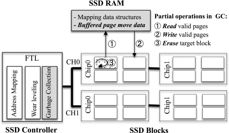
As illustrated in Figure 1, the SSD controller integrates the flash translation layer (FTL) supporting GC operations. In general, a GC process can be fulfilled with three steps: (1) Read : read valid pages from the GC target block to the SSD cache; (2) Write : write the valid pages to a free block from the cache; (3) Erase : erase the GC target block to reclaim the space.1 In fact, garbage collection is the most expensive operation in SSDs, and Erase accounts for a major part of time in a GC process [9, 11, 17]. This is due to both write and read requests targeting at the same channel or the same chip cannot be served when performing GC, which must place negative effects on I/O responsiveness of incoming requests [1].
Specially, a long tail is observed in the distribution of I/O latency resulted by completing GC requests, which must impact the real-time andquality of service (QoS) requirements of I/O services [13]. Regarding this issue, Wu and He [26] offered an approach to suspend the undergoing GC operation while a read request is coming for boosting read responsiveness, but the write performance can still be affected by the GC operations. Lee et al. [16] assign a higher priority to normal I/O requests over GC operations so it will suspend GC operations when a new I/O request arrives. Simply putting off the GC requests as low-priority tasks may offset their negative effects, but it may lead to unexpected performance degradation. This is because I/O requests should be eventually blocked and wait for the completion of GC to recycle space, when the free SSD space is not enough [12].
Then, Kang et al. [11] proposed a scheduling method using reinforcement learning to carry out the best fit GC actions between two I/O requests. Gao et al. [4] presented a cached GC scheme. This scheme first reads valid pages from the GC target block to the SSD cache and suspends writing the buffered data to SSD blocks until there is an idle interval between two requests. However, the GC operations affect not only the next I/O request, they might bring about negative effects on a set of incoming I/O requests. Therefore, it is better to dispatch GC requests by considering the idle state among multiple incoming requests. More importantly, these approaches failed to take the factor of free space demand of future I/O requests into account. For instance, it is expected to have more erase operations for reclaiming space if there will be intensive write requests.
To roundly address the issue of reducing the average I/O response latency caused by fulfilling GC requests, this article proposes a I/O intensity-aware scheme for adaptively carrying out partial GC operations. The basic idea is to conduct relevant partial GC operations, according to the forecast I/O intensity and the write ratio of requests in upcoming time windows. Specifically, we will assemble partial GC operations, i.e., Read or Write or Erase , and dispatch them together in future idle time slots2 of I/O processing, even if such operations are not involved to the same GC request. In brief, it makes the following three contributions:
- We propose an approach using Fourier transform [18] to predict the I/O intensity of target application in the near future. Then, a number of (partial) GC operations can be concentrately dealt with at the time slots having sparse I/O requests. As a result, the negative effects of GC can be confined to these time slots, as the number of affected normal I/O requests will be limited.
- We build a mathematical model to figure out what partial GC operations are preferred in a specific idle time slot to further minimize the I/O response latency. The factors of the SSD use state, the predicted I/O intensity, and the read/write ratio have been taken into account to determine the desired types and quantities of partial GC operations in specific idle time slots.
- We offer preliminary evaluation on several disk traces of real-world applications. As measurements indicate, our proposal can adaptively dispatch partial GC operations and then effectively cut down the negative effects caused by GC operations. Especially, the I/O response time and the long-tail latency can be noticeably cut down by 20.8% and 19.1% on average, compared with state-of-the-art approaches.
The rest of article is organized as follows: The related work and motivations are shown in Section 2. Section 3 describes the proposed partial GC scheduling. Section 4 presents the evaluation specifications. The article is concluded in Section 5.
2 BACKGROUND AND MOTIVATION
2.1 Related Work
Garbage collection and resource contention on I/O buses (channels) of SSDs will block all incoming read/write requests to the same I/O buses, which must bring about greater turnaround time for these requests [10]. To be specific, the first two partial operations of GC (i.e., Read and Write ) block the whole channel, and the last partial operation of Erase exclusively occupies the target chip [4, 10]. To minimize the negative effects on I/O latency caused by garbage collection, it is expected to either complete GC operations within less time [7, 23, 25] or place a higher priority to blocked I/O requests [1, 14, 26] or perform GC operations in the idle time intervals [4, 9, 11, 16].
To speed up GC processes, Wu et al. [25] and Hong et al. [7] have successively proposed fast garbage collection methods after exploring copyback error characteristics on real NAND flash chips. Shahidi et al. [23] introduced a novel parallel GC strategy in SSDs that aims to increase plane-level parallelism during GC. Choi et al. [1] proposed an I/O-parallelized GC scheduling technique, which uses the idle planes during GC to serve the blocked I/O requests. Moreover, Jung et al. [9] proposed two garbage collection policies for operating collectively to move GC operations from busy periods to idle periods. Unfortunately, the prediction of idle times in I/O workloads is challenging, and sometimes workloads do not have sufficiently long idle time slots for dealing with all GC requests [16]. This situation becomes even worse if the applications may change their storage access behavior at different runs or phases [11].
Considering two I/O requests may have an idle interval, but it is not enough for completing a GC request, Choudhuri et al. [2] proposed GFTL, which adopts performing partial GC to guarantee fixed upper bounds in the latency of storage access by eliminating the source of non-determinism. After that, Zhang et al. [28] introduced Lazy-RTGC to support partial garbage collection for providing the guaranteed system response time. Similarly, Kang et al. [11] presented a GC scheduling method on the basis of reinforcement learning to predict the idle time interval for conducting partial GC operations. It makes a prediction after processing each I/O request if available SSD space becomes not enough. Thus, it can timely conduct relevant partial GC operations of page move ( Read & Write ) and Erase with an adaptive manner to reduce the long-tail latency of I/O requests. Gao et al. [4] proposed a mechanism to cut down the overhead of page move in GC processes. It buffers valid pages of GC target block in SSD cache (i.e., Read ), and the buffered data will be flushed to the SSD cells when the device becomes idle (i.e., Write ).
Besides, Lee et al. [16] offered a technique, which can pipeline internal GC operations to merge them with pending I/O requests whenever possible, for reducing the negative effects of GC. Hahn et al. [5] proposed a just-in-time ( JIT ) GC technique to avoid unnecessary GC operations. It only triggers GC operations to reclaim SSD space if really needed. Yan et al. [27] designed and implemented TTFLASH, which can eliminate GC-induced tail latencies by avoiding GC blocked I/O requests with several novel strategies, including plane-blocking GC and rotating GC. But, it does need supports of special SSD internal advancements, such as capacitor-backed RAM and powerful controllers. Cui et al. [3] introduced ShadowGC, which regards the flash pages having dirty copies in the write buffers on both the host side and the SSD side as shadows. They designed ShadowGC to specially reclaim the shadow pages for performance.
There are commonly two kinds of approach to disclose idle time slots (or even idle time window) for GC operations. Some existing work regards a time window consisting of not many requests as an idle window [5, 9]. Other related work identifies idle time slots by mainly analyzing two adjacent requests [4, 11, 16]. For example, in the Cached-GC scheme proposed by Gao et al. [4], an idle time slot is found if if there is no I/O request after completing the current one. Then, the buffered valid data will be flushed to the SSD blocks. However, performing (partial) GC operations affects not only the next request, it may place negative effects on multiple incoming requests. This becomes especially true if the incoming requests are relatively intensive.
2.2 Motivations
Exploiting idle time intervals between two I/O requests for timely carrying out (partial) GC operations has been proposed to minimize GC overhead [4, 11]. But, the prediction of the length of idle time interval between two I/O requests is rather difficult. A failure prediction of an idle time slot between two requests must cause negative effects on incoming I/O requests.
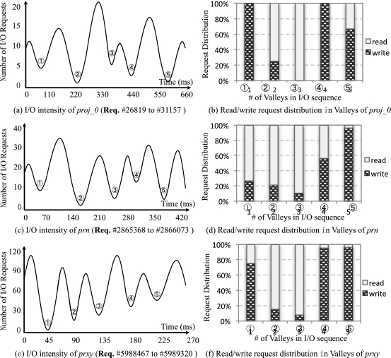
Then, we have analyzed I/O access frequency of some real-world applications by using Fast Fourier Transform (FFT) [24]. Figures 2(a), 2(c), and 2(e), respectively, demonstrate the I/O intensity of part of I/O sequence in the benchmarks of proj_0, prn, and prxy, which are the disk traces of real-world applications collected by Microsoft Research Cambridge [22]. In the figures, the X-axis represents the time line, and the Y-axis indicates the I/O frequency. As seen, the I/O frequency has multiple periodicity, and the valley areas (circled with numbers in the figure) imply that such time slots most likely have sparse I/O requests.
Observation I: I/O frequency of some applications does have regularity. Therefore, GC requests can be processed if the time intervals have been predicted holding sparse I/O requests.
After that, we have further explored the characteristics of read/write distribution in different valleys of the I/O sequence of selected traces, as shown in Figures 2(b), 2(d), and 2(f). Obviously, the ratio of read/write requests in different time slots is significantly diverse. Specially, read requests account for a major part of I/O workloads in some cases, though the selected traces are write-intensive.
On the basis of the characteristics of read/write distribution, it should perform the best fit partial GC operations. For example, we must do Erase of GC for reclaiming space, if SSD available space is not enough and a major part of incoming I/O requests are write requests. On the other side, we preferentially conduct lightweight partial GC operations, i.e., Write or Read , to minimize long-tail latency if the most of incoming requests are read requests.
Observation II: Applications have different read/write ratio at different stages of execution. It is expected to carry out fit partial GC operations by also considering the characteristics of incoming requests (e.g., read or write).
Such observations motivate us to complete GC requests, by taking the I/O characteristics and the SSD use state into account. (1) We carry out partial GC operations at the time slots having less I/O workloads to effectively reduce the number of requests affected by GC operations. (2) We assemble and dispatch partial GC operations belonging to the different GC requests by considering several factors, such as the I/O characteristics of incoming requests, to ultimately minimize the long-tail latency of I/O requests.
3 I/O INTENSITY-AWARE PARTIAL GC SCHEDULING
3.1 Overview
Figure 3 shows the high-level overview of the proposed approach of low I/O intensity-aware partial GC scheduling. Clearly, it dispatches partial GC operations to be processed at the time intervals having sparse I/O requests for reducing the number of requests that are affected by GC operations. Section 3.2 will show the details on disclosing future idle time slots by analyzing the history of I/O events in the application.
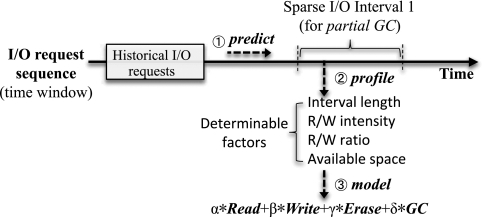
Moreover, it assembles partial GC operations by referring to several determinable factors, such as read/write ratio and the length of sparse I/O interval, for minimizing the negative effects of GC operations (e.g., long-tail latency). Section 3.3 will presents the specifications on assembling partial GC operations on the basis of the factors of I/O characteristics and the SSD use state.
3.2 Predicting I/O Intensity
As mentioned, there may be periodic read and write requests in the I/O sequence of application. Then, it is expected to avoid performing GC when I/O is intensive, as it might cause a significant delay for subsequent requests. In our scenarios, more specifically, we do not intend to predict what are the future ones in the time series of I/O requests, but prefer to know future idle time slots that have a relatively smaller I/O access frequency. Then, we can carry out (partial) GC operations without many delays on incoming I/O requests. Among many existing prediction techniques for time series data, Fourier transform is commonly used to identify the components with periodic volatility [18, 19]. Consequently, we take advantage of Fourier transform to unveil the periodicity of I/O frequency and then to purposely find time slots with low I/O access density.
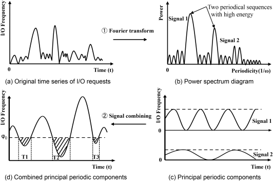
In fact, Fourier transform is originally introduced for decomposing complex synthetic signals and unveiling periodic components with high signal strength in a synthetic signal. That is to say, Fourier transform can represent a square integrable function of $f(t)$ as a series form of many trigonometric functions (see in Equation (1)). Then, the function of $f(t)$ in the time domain can be correspondingly expressed as the sum of the sine and cosine functions in the frequency domain, as indicated by $F(\omega)$ in Equation (2). Note that we do not create equations for our purpose; both equations are standard expressions of Fourier transform [18].
In our context, the intensity of I/O workload is treated as a signal, and Fourier transform is utilized to explore the possible periodic volatility of I/O intensity. Figure 4 demonstrates the process of disclosing time slots that have a small number of I/O requests among periodic volatility. First, the history of I/O request sequence can be expressed as Function $f(t)$ in the time domain (Figure 4(a)). Next, it is able to obtain the power spectrum of the sequence by using Fourier transform, and to extract several periodic signals with higher power energy (Figures 4(b) and 4(c)). After that, we can disclose periodic characteristics of I/O requests and then set a threshold (i.e., $\psi _0$ in Figure 4(d)) to determine trough areas (i.e., the shade areas in the figure), where hold sparse I/O requests.
Consequently, it is possible to predict the position and length of idle time slots in the next time window by following the disclosed patterns from the occurred I/O requests in the current time window. Thus, we can do (partial) GC operations in such slots to limit the number of I/O requests affected by GC, and then to guarantee I/O responsiveness.
3.3 Assembling and Scheduling Partial GC
Note that a GC process generally consists of Read , Write , and Erase operations, and it is not mandatory to complete these three partial operations at once [11]. Same as Cached-GC [4], our design is built on the top of the assumption that the SSD cache is dependable.3 In other words, it reads the valid data into the buffer, and the buffered data would not get lost in the case of a sudden power outage while SSD has large capacitors.
Our approach intends to assemble such partial operations even though they are not associated with the same GC request, by referring to the factors of characteristics of incoming I/O requests and the state of SSD use. To direct assembling and scheduling partial GC operations from case to case, we construct a mathematical model. Assuming we have an idle time interval for carrying out partial GC operations, and we aim to yield a minimum time cost after finishing certain (partial) GC operations, as demonstrated in Equation (3).
Similar to the reservoir problem, it is not expected to result in more waiting I/O requests on the SSD channels after certain (partial) GC operations. Then, we basically regard that the time cost of such GC operations is relating to the number of accumulated waiting I/O requests caused by completing them. Specifically, we first let $I_{in}$ as the number of arrived I/O requests per second in the target time interval, and the channel is unavailable while completing a specific operation (i.e., $T$), so the total amount of accumulated I/O requests is $I_{in} \times T$ after the specific operation. Once the SSD channel is able to process I/O requests, we set $I_{out}$ as the processing throughput of the SSD channel. That is to say, it needs the time of $T^{\prime }$ for satisfying all accumulated I/O requests resulted by completing (partial) GC operations, and we thus argue that Equation (4) is workable. Finally, we can obtain the time cost of completing a relevant operation (e.g., a partial GC operation or a full GC operation), as illustrated in Equation (5).
As illustrated in Equation (5), the time cost of $T_C$ has linear relationship with $T$. That is, $T_C= k \cdot T$, where $k$ is a constant. But, it has nonlinear relationship with $\lambda$, and the larger $\lambda$ implies the larger time cost for completing a (partial) GC operation.
Specially, in a GC process, both Read and Write will block the whole SSD channel, but Erase only delays the I/O requests onto the target SSD chip of channel. Assuming we have multiple chips in a channel, therefore, Equation (3) can be simplified to Equation (6).
Since we intend to utilize the idle time for (partial) GC operations as much as possible, the constraint defined in Equation (7) should be ensured. The sign of inequality is “$\ge$” in this constraint, otherwise it will not perform any GC-relevant operations, as the case of no operation can yield a minimal $T_{all\_C}$ as 0.
Our main purpose is to avoid time-consumed full GC operations to reduce the number of delayed incoming I/O requests, so such operations are performed if-and-only-if the available SSD space is less than a predefined hard threshold. Then, the number of required full GC operations can be obtained by following Equation (8).
Equation (8) ensures that the available space must be greater than the predefined hard threshold of $\phi ^{*}$, after performing Erase operations on erasable blocks that do not have any valid data or full GC operations on normal blocks that hold some valid data. On the other side, the number of Erase should be confined as the following equation:
In addition, the SSD cache (i.e., the page buffer), which is dedicated for temporarily holding the valid pages in GC processes, has limited capacity. The difference between the count of Read and the count of Write of GC in the time slot should be confined to the available cache space. Let $U_{all}$ representing the total pages of cache for holding valid pages in GC, and $U_\theta$ is the available pages of cache before processing I/O requests in the time slot of $\theta$. Therefore, we can obtain the constraint on cache use for correctly performing Read or Write operations in the time slot of $\theta$, as illustrated in Equation (10).
Finally, as summarized in Equation (11), the solution to the task of assembling partial GC operations is to obtain the minimal value of $z$ by following the aforementioned constraints to imply the best cost-performance measure.
subject to:
In fact, seeking the minimal value of $z$ is a general integer linear programming problem, which has only four decision variables. The next section will show our approach obtaining the expected values of decision variables.
3.4 Model Implementation
Because an existing Fast Fourier Transform implementation is used to predict the idle time slots,4 this section ignores its implementation details. After the length of idle time slot is disclosed, we use Algorithm 1 to yield the outcomes of our assembling model for directing partial GC operations in the explored idle time interval.
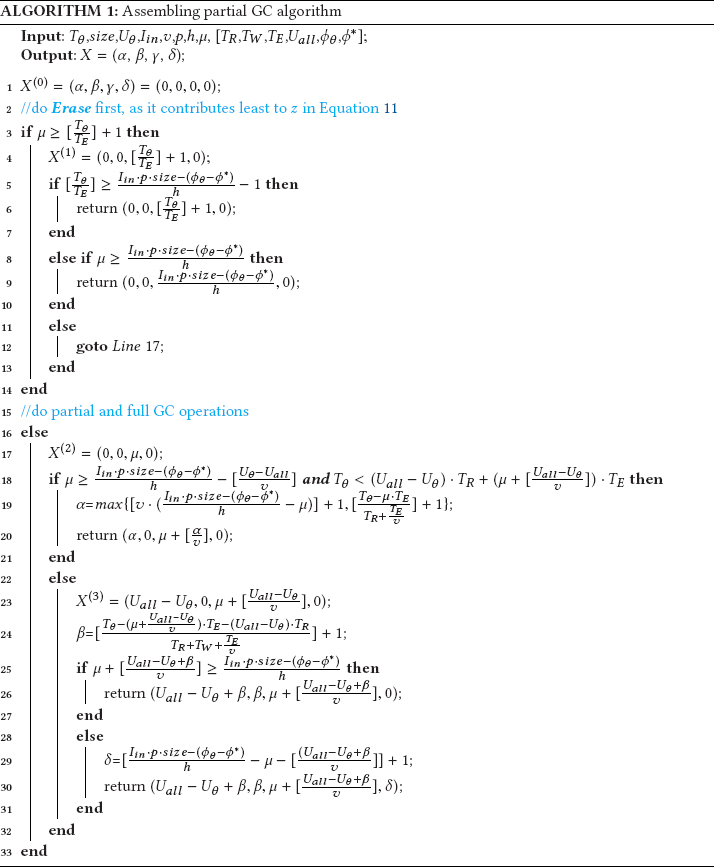
Besides the runtime parameters that are derived from the historical requests, the pre-defined parameters that are shown in the square brackets are also fed to our algorithm. Then, to yield the minimum value of objective function shown in Equation (11), we first erase the direct erasable blocks first (whose valid pages have been moved to the SSD cache), as illustrated in Lines 3-14. Next, Lines 17-21 cope with Read operations, because they contribute less to the value of $z$ in Equation (11), and may form direct erasable blocks for next rounds of processing. After that, it flushes the cached data to the SSD blocks to free cache space (i.e., Write ), as presented in Lines 23-27. Finally, it must carry out full GC operations if the free space is still not enough, as seen in Lines 29-30.
4 EXPERIMENTS AND EVALUATION
4.1 Experiment Setup
Considering SSD controller has limited computation power and memory capacity, we conducted tests on a local ARM-based machine. This machine has an ARM Cortex A7 Dual-Core with 800MHz, 128MB of memory and 32-bit Linux (ver 3.1). We have performed trace-driven simulation with SSDsim (ver2.1), which has a diverse set of configurations, and then been widely employed in many studies for measuring the performance of SSD systems through running simulation tests [8].
We have implemented our proposal as a part of flash transfer layer (FTL) and integrated it with SSDsim for enabling adaptive scheduling on partial GC operations. Table 1 shows our settings of SSDsim in tests. To reflect the impact of GC, the simulated SSD is aged to that with 80% of its capacity being used before running traces, and the page buffer is set as 128 pages (1 MB in total) by referring to the related work [4]. Specially, the read requests are never purposely delayed, and the time limitation to service the write requests is set as 5,000 ms by referring to Reference [35].
| Parameters | Values | Parameters | Values |
|---|---|---|---|
| Channel Size | 16 | Read latency | 0.075 ms |
| Chip Size | 4 | Write latency | 2 ms |
| Die Size | 2 | Erase latency | 15 ms |
| Plane Size | 2 | Transfer (Byte) | 10 ns |
| Block per plane | 256 | Write deadline | 5,000 ms |
| Page per block | 256 | GC Threshold | 5% |
| Page Size | 8 KB | FTL Scheme | Page level |
| Page Buffer | 128 pages (1MB) | ||
| Note: LUN traces do not have many GC operations with the default settings because of small size of footprint; we thus set channel size as 2 for them. |
|||
We selected eight block I/O traces for our evaluation, and Table 2 reports the specifications on the selected traces. Among them, three traces are from Microsoft Research Cambridge, which is afforded by multiple enterprise servers for different applications [22]. Another three write-intensive block I/O traces of 2016021614-LUN0, 2016021615-LUN0, and 2016021616-LUN1 (labeled as lun1-1, lun1-2, and lun1-3) are collected from an enterprise VDI (Virtual Desktop Infrastructure) [15]. Moreover, two YCSB RocksDB traces on SSDs of ssdtrace-01 and ssdtrace-02 (labeled as YCSB-01, and YCSB-02), which have been recently collected in the SNIA IOTTA Repository [29], are also employed as the input data in our tests. Each trace (size $\sim$ 1 GB) in the YCSB collection corresponds to different segments of the original blocktrace file, and all YCSB traces have similar I/O access features [30]. Due to this fact, we only used the first two traces to represent all traces in our tests.
| Traces | Req # | Wr Ratio | Wr Size | Total Wr Size | Max/Avg INT |
|---|---|---|---|---|---|
| proj_0 | 4,224,524 | 87.5% | 40.9KB | 144.3GB | 249.1/1.4ms |
| prn_0 | 5,585,886 | 89.2% | 9.7KB | 45.9GB | 100.1/1.0ms |
| prxy_0 | 12,518,968 | 96.9% | 4.7KB | 53.8GB | 183.2/0.4ms |
| lun1-1 | 867,967 | 52.8% | 11.3KB | 4.9GB | 1,315.2/4.1ms |
| lun1-2 | 1,073,405 | 73.1% | 7.6KB | 3.9GB | 6,488.8/3.3ms |
| lun1-3 | 749,806 | 61.5% | 8.8KB | 5.7GB | 944.1/4.7ms |
| YCSB-01 | 13,178,499 | 2.5% | 716.7KB | 221.5GB | 24,484.7/8.1ms |
| YCSB-02 | 13,178,150 | 2.5% | 714.8KB | 224.4GB | 26,003.6/8.3ms |
| Note: All traces are repeated twice to make a large amount of write data. In which, the metrics of Wr Size and Total Wr Size indicate the average write size and the total write size, respectively. Besides, the minimum interval is 0 ms in all selected traces. |
|||||
Our proposal takes advantage of Fourier transform to analyze the historical I/O requests in the latest time window(s), for predicting the intensity of future I/Os. After sensitive tests (refer to Section 4.2.7), we have fixed some parameters in a round of Fourier transform. The number of requests in every 15 ms is referred to as a point, and we term this 15 ms as the length of point. There are 4,096 historical points in the training set for predicting the following 2,048 points in the coming time window. That is to say, the length of time window is 15 ms$\times$2,048=30.72 seconds in the our tests. The parameter of $\psi _0$ shown in Figure 4(d), which is used to identify idle slots, is set as 0.35.
To yield fit combinations of partial GC operations from time to time, it analyzes 256 most recently occurred I/O requests for deciding the runtime parameters introduced in Equation (11). For example, the number of incoming requests of $I_{in}$ can be duly counted for assembling partial GC operations. Besides, the average size of reclaimed free space (labeled as $p$) and the average number of page move in each GC operation (labeled as $v$) are calculated as the average released space of 32 recent GCs.
Besides the proposed approach (labeled as Demand), the following GC scheduling schemes were also used as comparison counterparts in tests:
- Baseline: which implies SSDs only support full GC processes, and GC operations will be immediately triggered if the available space becomes insufficient.
- Cached-GC [4]: which is a representative GC scheduling method for separately dealing with Read and Write operations during a GC process. It first buffers valid pages of GC blocks to the SSD cache and then exploits idle time to flush them onto SSD blocks to minimize negative effects caused by GC operations.
- RL-GC [11]: which is reinforcement learning-assisted GC, for reducing the long-tail latency of I/O requests. Specifically, RL-GC uses the reinforcement learning approach to explore idle time slots between two I/O requests for carrying out one or more operations of page move and Erase . RL-GC might be the most related work on adaptive GC scheduling by adopting three levels of GC threshold. In the cases of the maximum level and the medium level of threshold, it conducts partial GC operations according to the current state. But, it will mandatorily execute certain partial GC operations if the SSD reaches the minimum level of GC threshold, even though there is no idle time interval.
- Erase Suspension [26]: which places a high priority to read requests for guaranteeing read responsiveness. In other words, it suspends the on-going erase operation for immediately servicing read operations, but it does not contribute to better responses to write requests.
- Arima [20]: which makes use of Autoregressive Integrated Moving Average (ARIMA) to analyze I/O access frequency of selected block I/O traces for predicting idle time slots in the near future. Then, it performs the proposed partial GC assembling and scheduling scheme in the predicted idle time slots. Because Arima is the most commonly used method for predicting the time series data, we employ it as another comparison counterpart to verify the effectiveness of Fourier transform in predictions of idle time slots.
4.2 Results and Discussions
To measure validity of the proposed partial GC scheduling mechanism that aims to reduce the negative effects caused by GC operations in SSDs, we employ the following two metrics in our tests: (a) average I/O latency and (b) I/O long-tail latency. This section also reports the erase statistics, the distribution of partial GC operations, overhead, and the prediction accuracy of our scheme. After that, we check the performance changes of our proposal with varying page buffer size and carry out sensitivity analysis on several tunable parameters in our model.
4.2.1 I/0 Response Time. The proposed GC scheme intends to perform the best fit assembled partial GC operations in idle time slots. Because the average I/O response time depends on the size of requests in the traces, it varies greatly when processing different traces. Therefore, we collect the normalized I/O response performance including the read latency, the write latency, and the overall I/O latency in this section, and Figure 5 shows the results.
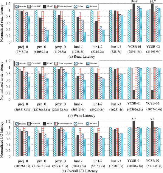
As seen, Demand brings about the least I/O response time in all traces, while Baseline performs the worst except for the two YCSB traces, because it does not enable optimization strategies on GC scheduling. While running two YCSB traces, the aggressive partial write operations in Demand interfere with foreground read requests, so Demand does slightly worse than Baseline in the measurement of read latency. More exactly, compared with the related work, our proposal can reduce the response time by 43.2% on average in our tests. We argue the reason is that CachedGC only flushes the buffered data to SSD blocks in the idle time, it fails to schedule Erase and Read operations to be processed in the idle time. Erase Suspension cannot benefit to write requests, as only the read requests have a high priority than GC operations, and Arima is good at the prediction of short-term stationary series and not adapted to our scenarios (see prediction accuracy in Table 3).
| Traces | # of Win. | FFT | ARIMA | ||
|---|---|---|---|---|---|
| Pred. slots | Hits (ratio) | Pred. slots | Hits (ratio) | ||
| proj_0 | 2,364 | 14,546 | 9,600(66.0%) | 15,702 | 9,690(61.7%) |
| prn_0 | 592 | 10,558 | 7,346(69.6%) | 12,194 | 7,882(64.6%) |
| prxy_0 | 592 | 16,254 | 11,668(71.8%) | 20,028 | 13,260(66.2%) |
| lun1-1 | 352 | 4,244 | 3,012(71.0%) | 7,856 | 5,044(64.2%) |
| lun1-2 | 352 | 5,532 | 3,870(70.0%) | 8,510 | 5,658(66.4%) |
| lun1-3 | 352 | 3,346 | 2,388(71.4%) | 6,350 | 4,062(63.9%) |
| YSCB-01 | 2,865 | 92,962 | 77,438(83.3%) | 169,306 | 131,812(77.8%) |
| YCSB-02 | 2,887 | 91,274 | 76,226(83.5%) | 172,408 | 133,170(77.2%) |
As the most related work, RL-GC must mandatorily complete certain page move s if the available space is inefficient. Our statistics on replaying the selected traces show that 4.1%-96.6% of page move s are mandatorily completed in RL-GC, which have delayed the coming normal I/O requests. More interestingly, RL-GC significantly performs the best in write performance but the worst in read performance after running the selected two read intensive traces of YCSB-01, and YCSB-02. This is because different from other GC scheduling methods that trigger (partial) GC operations before servicing a write request, RL-GC adopts “read-initiated GC triggering” [11], and it may carry out (partial) GC operations after fulfilling read requests.
In brief, we have verified that assembling partial GC operations and completing them in idle time slots can minimize the negative effects of GC operation and then noticeably cut down the latency in I/O processing, in contrast to the comparison counterparts.
4.2.2 Long-tail Latency. To reduce the long-tail latency is another primary target of the proposed scheme, Figure 6 compares the long-tail latency (in CDF) for all I/O requests after running the selected benchmarks. The figure shows that our proposed method exhibits better measurement of long-tail latency than that using other three comparison counterparts.
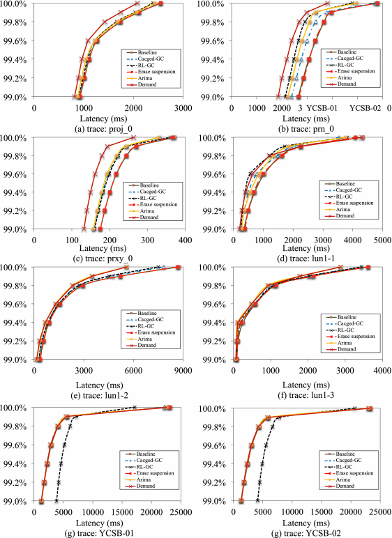
Different from other three schemes, Baseline causes too large latency, since it does not adopt any optimization strategies to mitigate the long-tail latency. Another interesting clue shown in the figure is that Demand does significantly reduce the long-tail latency by 12.8%, 34.5%, 22.7%, and 10.2% at the 99.99th percentile, compared with the state-of-the-art schemes of CachedGC, RL-GC, Erase Suspension, and Arima, respectively.
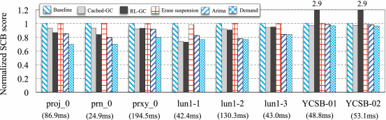
To further disclose how the proposed method reduces or mitigates the effects of long-tail latency, we define the SCB (Slowdown Caused by Blocking) score for a given I/O request, as the time difference between the practical response time and the theoretical response time. In which, the practical response time is the completed time in the simulation tests, and the theoretical response time is the sum of the arrival time and the required time for doing the read/write request. This metric is referring to Reference [34] and can give the theoretical slowdown of read/write requests caused by waiting in the I/O queue.
Since the SCB scores varies from case to case after running the benchmarks, we present the normalized measurements in Figure 7. As seen, Demand can reduce the SCB score by 18.9%, 10.5%, 56.8%, 18.6%, and 6.0% on average, in contrast to Baseline, Cached-GC, RL-GC, Erase-suspension, and Arima. It further verifies our proposal can efficiently remit I/O congestion caused by GC-relevant operations to decrease the waiting cost of reads and consequently minimize the overall I/O time.
In summary, Demand assembles partial GC operations in an adaptive manner by referring to several determinable factors for confining the negative effects of GC to a small number of incoming I/O requests. Thus, it can reduce the number of blocked I/O requests caused by GC operations and then show better long-tail latency than related work.
4.2.3 Erase Statistics and Available Space. Figure 8(a) presents the total erase counts caused by running the selected benchmarks while using different GC scheduling schemes. As reported, the proposed scheme of Demand does introduce the largest number of erase operations in all selected GC scheduling schemes. This is because Demand intends to carry out (partial) GC operations for reclaiming free space as much as possible if there is an idle time slot. That is to say, our proposal should yield a larger available space after running the benchmarks, compared with other schemes. While using Arima and Demand, both partial GCs (triggered in idle time slots after the soft threshold of GC is reached) and normal GCs (triggered compulsively after the hard threshold of GC is reached) lead to erase operations, so their bars are labeled as two parts. As seen in Figure 8(a), the blank part indicates the erases caused by normal GCs, and the colored part means the erases resulted by partial GCs. For example, in the case of proj_0, 54.8% and 100% erase operations are introduced by partial GCs when using Arima and Demand. This is the reason why Demand can yield the best I/O response time and the long-tail latency after replaying proj_0, as the negative effects of GC can be minimized.
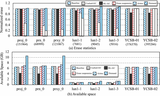
Figure 8(b) presents the results of the available space introduced by varied GC schemes. Clearly, Demand does have the largest available space in all cases, because our proposal has completed many erase operations in advance, which contribute to recycling more free space. More importantly, we have surveyed how much the possible available space brought about by the selected related work if a number of Erase operations can be additionally performed. We take running proj_0 with Cached-GC as an example. On the one side, Cached-GC yields a reduction of Erases by 2,057 in contrast to Demand. On the other side, Demand achieves 10.6 GB free space, but Cached-GC gets only 6.6 GB free space after running the benchmark. It is true that Cached-GC will ideally obtain free space up to 10.7 GB (only slightly greater than 10.6 GB) after additionally conducting 2,045 erases. However, we should not ignore the overhead of such erases in practice, and one erase cannot generally recycle a whole block space, as there might be some valid pages in the target block. In conclusion, we emphasize that more erase operations introduced by our proposal is not a negative result, but rather a positive outcome.
4.2.4 Partial GC Operation Distribution. Our approach adaptively carries out partial GC operations, according to the factors of I/O characteristics and the use state of SSD. Figure 9 illustrates the distribution of partial GC operations after running the selected I/O traces. In the figure, the X-axis represents the sequence of time window, and Y-axis means the operation distribution in percentage. Because different benchmarks have different total execution time, the length of time window varies from trace to trace.
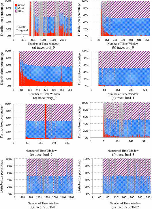
For most of benchmarks, the distribution of partial GC operations keeps changing over time while the determinable factors make a difference. Specially, for the benchmarks of lun1-1 and lun1-2, both Read and Write keep a large and stable percent during runtime. This is due to both of them not having many frequent write addresses (only 6.9% and 7.0% addresses have been written twice or more). So, a large number of valid pages are expected to be moved during garbage collection when the available space is not enough.
Note that there is no partial GC operation at the early stages of running the benchmarks, as the device holds more than 8% free space at beginning. This is also the reason for no partial GC operations in some time windows of running the benchmarks at late stage (i.e., the interspace in distribution figures). After a while, it preferentially performs erase operations for reclaiming the space on the blocks having no valid pages, so the percentage of Erase is almost 100%, even though the absolute number is only 1 or 2. As time went by, the numbers of Read and Write increase, and both kinds of operations take a major part of all operations when running the most benchmarks at the late stage.
Another noticeable information shown in Figure 9 is about no partial GC operation of Erase after running YCSB-01 and YCSB-02, which implies all erase operations are completed in normal GCs (that are also previously illustrated in Section 4.2.3). This is because larger read/write requests in both YCSB traces require longer time to be completed, even though the time interval between two requests is not small. Then, it does not have enough idle time for completing the partial GC operation of Erase .
In brief, it verifies our approach can predict the position and length of idle time slots for carrying out fit partial GC operations in the different time windows by considering several determinable factors, such as the characteristics of incoming requests.
4.2.5 Model Overhead and Prediction Accuracy. The main space overhead of the proposed approach is on the valid page buffer in SSD cache. In the evaluation tests, the size of valid page buffer is set as 1,024 KB for keeping 128 valid pages.
The SSD controller is responsible for predicting idle time slots and optimizing partial GC combination. We have then measured its time needed to predict idle time slots and the time needed to assemble partial GC operations. In other words, the requests in the I/O queue cannot be dispatched to SSD blocks for end when the SSD controller is dealing with modeling computations. Note that although this section only discusses the time overhead, such overhead does bring about side effects on I/O responsiveness by delaying the processing on incoming I/O requests, and relevant results have been reported in Sections 4.2.1 and 4.2.2.
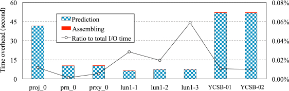
After running the benchmarks on the ARM-based platform, Figure 10 reports the time overhead caused by FFT computations (i.e., Prediction) and assembling computations (i.e., Assembling). According to our measurements shown in the figure, our proposal results in time overhead between 6.6 and 52.0 seconds after replaying the selected block I/O traces. This corresponds an average of 3.6 $\mu$s per I/O request, or less than 0.06% of the overall I/O time. Then, we consider that the time overhead caused by the proposed prediction and assembling approach is acceptable, even though our experiments are done on an ARM platform.
Furthermore, we have recorded the number of prediction hits on idle time slots to show the accuracy of the prediction methods of FFT and ARIMA. We define a prediction hit as the case of the forecast I/O intensity is not 10% higher than the actual one. Table 3 presents the results of the prediction accuracy while using both FFT and ARIMA. Clearly, in contrast to ARIMA, the adopted FFT method can yield higher accuracy by 9.8% on average after running the selected traces.
4.2.6 Scalability with Varied Size of Cache. This section reports the scalability of the proposed Demand schemes on varied sizes of SSD cache. Figures 11(a) and 11(b), respectively, disclose the normalized I/O response time and the number of buffered pages introduced by Read operations, while the proposed Demand scheme runs with the SSD cache size varying from 256 K to 4 M.
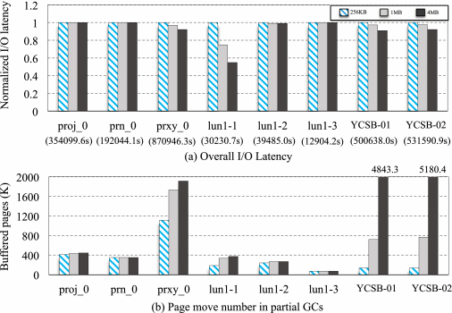
On the one side, the I/O response time keep decreasing while the SSD cache becomes larger after replaying prox_0, lun1-1 and two YCSB traces. This is because a large size of SSD cache can temporarily buffer more data pages in partial GC processes, and the negative impacts of GC can be consequently reduced. On the other side, it does not make obvious difference when replaying the traces of proj_0, prn_0, lun1-2, and lun1-3 when the cache size becomes larger. In such cases, we have observed that the large size of cache is not filling up with the read data introduced by Read operations. As shown in Figure 11(b), the buffered data pages remain roughly unchanged after running these traces with varied sizes of cache.
Generally, a capacitor is equipped to ensure the SSD page buffer keeping persistent, for fighting against a power failure, and a larger memory buffer normally accompanies with a larger capacitor in SSDs. Then, we have analyzed the capacitor requirements according to different size of page buffer in SSDs, as well as the energy cost of capacitor.
4.2.7 Sensitivity Analysis. To further understand the impact of the several tunable parameters, which are critical to the performance of the proposed approach, we run benchmarks to investigate their impact. Three tunable parameters affect the performance when running the benchmarks: (1) the size of time window in the process of analyzing I/O intensity, (2) the threshold of $\psi _0$ to classify the idle time slots after fast Fourier transform, (3) the soft GC threshold for triggering partial GC operations. Specially, we change the length of time point to indicate varied size of time window.
In the tests, we vary three parameters indicating a large range of possible scenarios. Then, the I/O response time with varied cases is recorded, as this metric is the most important indication of I/O responsiveness. Figure 12 shows the sensitive analysis of critical parameters.
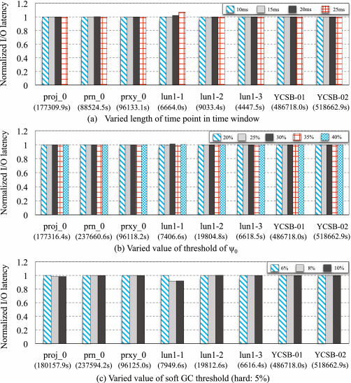
In Figure 12(a), we see a relative greater length of time point does not benefit to the reduction of I/O latency; the length of time points 25 ms and 20 ms do not outperform the case of 15 ms in all traces. This is because a large length of time point can cut down the number of operations of fast Fourier transform, but it may increase the time of a GC processing cycle. As shown in Figure 12(b), the varied size of threshold of $\psi _0$ in the range of [0.2, 0.4] does not noticeably impact I/O responsiveness, though 0.3 and 0.35 of $\psi _0$ yield a slight improvement. Figure 12(c) shows how varied soft GC thresholds affect the I/O responsiveness. As seen, large soft GC thresholds can yield a performance improvement, since more GC operation can be completed in advance if there is an idle time. But if the soft GC threshold is too large, it will aggressively cause more GC operations, which may shorten the SSD lifetime.
4.3 Case Studies
4.3.1 Case Study on Sub-block Erase over 3D-NAND. Considering the block size becomes larger in recent 3D NAND flash chips, the page move overhead in the GC process keeps increasing [36]. To improve the system performance by reducing GC overheads and boost the device reliability/lifetime, some studies are proposed to make flash chips supporting “sub-block erase” to cut the page move overhead. In general, the functionality of sub-block erase is enabled by redundant hardware or software emulated free space as the isolation layer [36, 37, 38]. This section carries out a case study to check the effectiveness of our proposal in the sub-block erase supported 3D-NAND flash memory.
Figure 13 demonstrates the results of I/O performance and erase statistics by using the newly proposed scheme and other selected related work on GC scheduling. As seen in Figure 13(a), Demand can decrease the overall I/O response time by 10.9%, 232.3%, 14.5%, and 5.5% on sub-block erase over 3D NAND flash memory, compared with the related work of CachedGC, RL-GC, Erase Suspension, and Arima, respectively. This proves the proposed GC scheduling method can work well on 3D-NAND with the feature of sub-block erase.
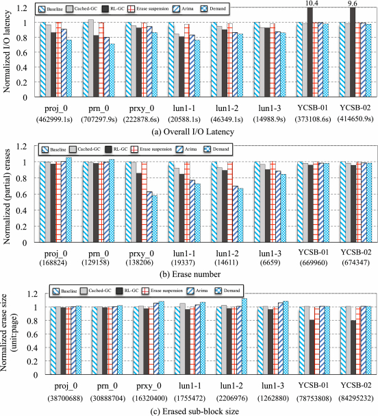
Note that, different from the tendency of erase statistics on conventional SSDs, Demand results in the least number of sub-block erases on average after running the selected traces with sub-block erase supports, as illustrated in Figure 13(b). This is because Demand will greedily trigger sub-block erases after the soft GC threshold reaches, and each erase process may deal with a large size of sub-block accompanying with more page moves, which are demonstrated in Figure 13(c).
4.3.2 Case Study on Worst-case of FFT Predictions. To check how much performance degradation occurs if FFT-based predictions do not work at all, we then use FFT to analyze the block trace of YCSB-02, which has the largest number of time windows among all selected traces and apply the predicted idle time intervals of YCSB-02 onto other block traces. That is to say, all selected block traces except for YCSB-02 do have unpractical predictions on idle time slots.
Since this case study aims to disclose the performance degradation caused by Demand in case the FFT-based predictions become useless, we only employ Baseline to be the comparison counterpart in this case study. Note that Baseline triggers RR operations regardless of the I/O intensity status, and Demand carries out (partial) GC operations Figures 14(a) and 14(b) separately present the relevant results of overall I/O latency and the erase statistics after replaying the selected traces.
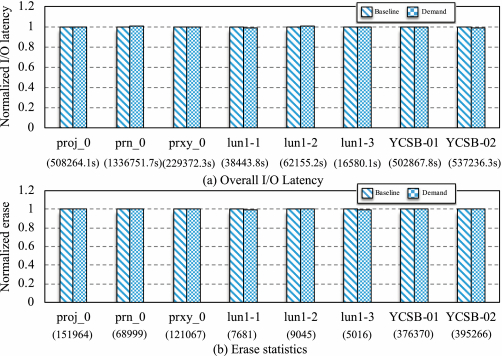
As shown the figures, Demand does slightly worse than Baseline by no more than 0.79% and 0.08% in the measures of the overall I/O time and the erase number, except for the case of YCSB-02. In the tests, we employ the FFT predictions of YCSB-02 for all traces except for YCSB-02, which lead to a very small performance drop. In brief, such results further verifies that the proposed partial GC scheduling method does not harm much even though with inaccurate predictions, in contrast to Baseline.
4.4 Summary
With respect to comparing conventional GC schemes and the proposed low I/O intensity-aware scheduling method, we emphasize the following two key observations: First , conducting (partial) GC operations in the time slots with less I/O requests can noticeably confine the negative impacts of GC to a limited number of I/O requests. Second , assembling partial GC operations based on the I/O characteristics and the SSD use state can effectively minimize the long-tail latency. But note that our proposal cannot outperform conventional methods for the cases in which I/O workloads do not have regularity. That is, our adopted FFT prediction method fails to correctly predict the idle time slots if the I/O workloads change dynamically in very short intervals.
5 CONCLUSIONS
This article has proposed a low I/O intensity-aware scheduling approach on partial GC operations for cutting down negative effects of GC in SSDs. To be specific, it first analyzes the history of I/O requests to forecast I/O periodicity of application by using Fourier transform. Then, it is possible to identify future time slots with less I/O workloads and to complete (partial) GC operations in such low I/O intensity slots. Consequently, the (partial) GC operations will not delay many incoming I/O requests and brings about less negative impacts on I/O responsiveness. Moreover, we have constructed a mathematical model to better utilize the idle time slots for minimizing the long-tail latency of I/O requests. This model considers several determinable factors, including I/O characteristics and the state of SSD use, to yield the types and relevant quantities of partial GC operations. After that, the assembled partial GC operations are supposed to be performed in a specific idle time slot.
Experimental results have shown that the proposed GC scheduling scheme can decrease the time needed for completing the I/O requests of benchmarks by 65.7% on average. Our measurements also illustrate the proposed approach can reduce the long-tail latency by between 3.8% and 39.1% at the 99.99th percentile, in contrast to the state-of-the-art GC scheduling schemes.
The current implementation of I/O intensity prediction does not work well if I/O patterns change very frequently in target applications. Therefore, we are planning to improve our prediction approach for dealing with bursty and dynamic I/O workloads (e.g., the applications running on distributed or cloud platforms) in our future study.
REFERENCES
- W. Choi, and M. Kandemir. 2018. Parallelizing garbage collection with I/O to improve flash resource utilization. In HPDC’18.
- S. Choudhuri and T. Givargis. 2008. Deterministic service guarantees for NAND flash using partial block cleaning. In CODES+ISSS’08.
- J. Cui, Y. Zhang, and J. Huang. 2018. ShadowGC: Cooperative garbage collection with multi-level buffer for performance improvement in NAND flash-based SSDs. In DATE’18.
- C. Gao, L. Shi, and Y. Di. 2018. Exploiting chip idleness for minimizing garbage collection–induced chip access conflict on SSDs. ACM Trans. Des. Automat. Electron. Syst.2018. DOI: https://doi.org/10.1145/3131850
- S. Hahn, J. Kim, and S. Lee. 2015. To collect or not to collect: Just-in-time garbage collection for high-performance SSDs with long lifetimes. In DAC.
- T. Hatanakay, R. Yajima, and T. Horiuchi. 2010. Ferroelectric (Fe)-NAND flash memory with batch write algorithm and smart data store to the nonvolatile page buffer for data center application high-speed and highly reliable enterprise solid-state drives. IEEE Solid-state Circ., 2010. DOI: https://doi.org/10.1109/JSSC.2010.2061650
- D. Hong, and J. Park. 2019. Improving SSD performance using adaptive restricted-copyback operations. In NVMSA’19.
- Y. Hu, H. Jiang, and D. Feng. 2013. Exploring and exploiting the multilevel parallelism inside SSDs for improved performance and endurance. Trans. Comput., 2013. DOI: https://doi.org/10.1109/TC.2012.60
- M. Jung, R. Prabhakar, and M. Kandemir. 2012. Taking garbage collection overheads off the critical path in SSDs. In Middleware’12.
- M. Jung, W. Choi, and M. Kwon. 2019. Design of a host interface logic for GC-Free SSDs. J. Technol. Comput. Aided Des., 2019. DOI: https://doi.org/10.1109/TCAD.2019.2919035
- W. Kang, D. Shin, and S. Yoo. 2017. Reinforcement learning-assisted garbage collection to mitigate long-tail latency in SSD. Trans. Embed. Comput. Syst.2017.
- B. Kim, H. Yang, and S. Min. 2018. AutoSSD: An autonomic SSD architecture. In ATC’18.
- S. Kim, J. Bae, and H. Jang. 2019. Practical erase suspension for modern low-latency SSDs. In ATC’19.
- J. Kim, K. Lim, and Y. Jung. 2019. Alleviating garbage collection interference through spatial separation in all flash arrays. In ATC’19.
- C. Lee, T. Kumano, and T. Matsuki. 2017. Understanding storage traffic characteristics on enterprise virtual desktop infrastructure. In SYSTOR’17.
- J. Lee, Y. Kim, and G. Shipman. 2013. Preemptible I/O scheduling of garbage collection for solid state drives. In J. Technol. Comput. Aided Des.2013. DOI: https://doi.org/10.1109/TCAD.2012.2227479
- J. Li, X. Xu, and X. Peng. 2019. Pattern-based write scheduling and read balance-oriented wear-leveling for solid state drivers. In MSST’19.
- N. Masters. 1995. Novel and Hybrid Algorithms for Time Series Prediction. John Wiley & Sons, Inc..
- S. Tashpulatov. 2013. Estimating the volatility of electricity prices: The case of the England and Wales wholesale electricity market. Energy Policy 60 (2013), 81–90.
- H. Nguyen, M. Naeem, and N. Wichitaksorn. 2019. A smart system for short-term price prediction using time series models. Comput. Electric. Eng., 2019. DOI: https://doi.org/10.1016/j.compeleceng.2019.04.013
- C. Matsui, C. Sun, and K. Takeuchi. 2017. Design of hybrid SSDs with storage class memory and NAND flash memory. In PIEEE’17.
- MSRC Traces. http://iotta.snia.org/traces/388.
- N. Shahidi, M. Arjomand, and M. Jung. 2016. Exploring the potentials of parallel garbage collection in SSDs for enterprise storage systems. In SC’16.
- H. Sorensen, D. Jones, and M. Heideman. 1987. Real-valued fast Fourier transform algorithms. In TASSP’87.
- F. Wu, J. Zhou, and S. Wang. 2018. FastGC: Accelerate garbage collection via an efficient copyback-based data migration in SSDs. In DAC’18.
- G. Wu and X. He. 2014. Reducing SSD read latency via NAND flash program and erase suspension. In FAST’14.
- S. Yan, H. Li, and M. Hao. 2017. Tiny-tail flash: Near-perfect elimination of garbage collection tail latencies in NAND SSDs. In FAST’17.
- Q. Zhang, Q. Li, and L. Wang. 2015. Lazy-RTGC: A real-time lazy garbage collection mechanism with jointly optimizing average and worst performance for NAND flash memory storage systems. ACM Trans. Des. Automat. Electron. Syst.2015. DOI: https://doi.org/10.1145/2746236
- Y. Gala, G. Moshe, and J. Shehbaz. 2021. SSD-based workload characteristics and their performance implications. ACM Trans. Stor.2021. DOI: https://doi.org/10.1145/3423137
- YCSB RocksDB SSD Traces. 2020. Retrieved from http://iotta.snia.org/traces/28568.
- MP5515. Retrieved from https://www.monolithicpower.com/en/mp5515.html.
- Samsung 970 EVO Datasheet. Retrieved from https://www.samsung.com/semiconductor/global.semi.static/Samsung_NVMe_SSD_970_EVO_Data_Sheet_Rev.1.0.pdf.
- F. Ulaby, E. Michielssen, and U. Ravaioli. 2010. Fundamentals of Applied Electromagnetics (6th ed.). Prentice Hall.
- M. Bouksiaa, and F. Trahay. 2019. Using differential execution analysis to identify thread interference. IEEE Trans. Parallel Distrib. Syst.2019. DOI: https://doi.org/10.1109/TPDS.2019.2927481
- B. Mao, S. Wu, and L. Duan. 2017. Improving the SSD performance by exploiting request characteristics and internal parallelism. J. Technol. Comput. Aided Des.2017. DOI: https://doi.org/10.1109/TCAD.2017.2697961
- T. Chen, Y. Chang, and C. Ho. 2016. Enabling sub-blocks erase management to boost the performance of 3D NAND flash memory. In DAC’16.
- H. Chang, C. Ho, Y. Chang. 2016. How to enable software isolation and boost system performance with sub-block erase over 3D flash memory. In CODES+ISSS’16.
- C. Liu, J. Kotra and M. Jung. 2018. PEN: Design and evaluation of partial-erase for 3D NAND-based high density SSDs. In FAST’18.
Footnotes
- 1We name these three steps as three partial operations of GC in this article. The first two operations are normally united as a page move operation [9, 17]. In the article, we use bold italic terms to stand for partial GC operations and normal terms for representing conventional operations.
- 2The terms time slot and time interval are used interchangeably in this article, and a time window contains multiple time slots.
- 3“The nonvolatile page buffer realizes a highly reliable operation even in a power outage,” by Hatanaka, 2010 [6].
- 4Refer to https://github.com/rshuston/FFT-C, but the function of memory leak checks is disabled for better responsiveness.
Jianwei Liao works for College of Computer and Information Science, Southwest University of China, and State Key Lab. for Novel Software Technology, Nanjing University, P.R. China. This work was partially supported by “National Natural Science Foundation of China (No. 61872299, No. 62032019, No. 61732019),” “Chongqing Graduate Research and Innovation Project (No. CYS20117),” “the Opening Project of State Key Laboratory for and Novel Software Technology (No. KFKT2021B06),” “the Capacity Development Grant of Southwest University (No. SWU116007),” and Chongqing Talent (Youth) (No. CQYC202005094).
Author's addresses: Z. Sha, J. Li, L. Song, J. Tang, M. Huang, Z. Cai, J. Liao (corresponding author), and Z. Liu, Southwest University of China, Chongqing, China, 400715; emails: shazb171318515@163.com, lijun19991111@126.com, mooncake1223@163.com, vigouroustang@outlook.com, hmin@swu.edu.cn, czg@swu.edu.cn, liaotoad@gmail.com, zhimingliu88@swu.edu.cn; L. Qian, Chengdu SGK Semiconductor Co, Ltd, Chengdu, China; email: qianlianju@163.com.
Permission to make digital or hard copies of all or part of this work for personal or classroom use is granted without fee provided that copies are not made or distributed for profit or commercial advantage and that copies bear this notice and the full citation on the first page. Copyrights for components of this work owned by others than ACM must be honored. Abstracting with credit is permitted. To copy otherwise, or republish, to post on servers or to redistribute to lists, requires prior specific permission and/or a fee. Request permissions from permissions@acm.org.
©2021 Association for Computing Machinery.
1544-3566/2021/07-ART46 $15.00
DOI: https://doi.org/10.1145/3460433
Publication History: Received September 2020; revised April 2021; accepted April 2021