1. Introduction
The Travelling Salesman Problem (TSP) is one of the most well-known and extensively studied combinatorial optimization problems by far. It has been used as a benchmark problem for new urban and navigation developments for decades. It asks to find the shortest (in terms of length, time, or custom cost) route that visits each vertex in a given set exactly once before returning to the starting vertex. Formally, it could be stated as follows: given a directed/undirected graph
with set of vertices
V and set of weighted edges
E, find the shortest path between start vertex
s and end vertex
e (
e could be same as
s for closed path) that visits each vertex of a given set
exactly once. It is equivalent to finding the minimum-cost Hamiltonian cycle in
G [
1]. It has many applications in ranging areas of geo-spatial sciences and GIS, like in vehicle routing, urban communication networking, public transport sequencing and scheduling, to name a few (please read [
2]). It has always been a great source of attraction from various other disciplines too, especially during the last three decades [
3].
The Generalized-TSP (GTSP) or Set-TSP or Travelling Politician Problem is one useful exemplary of the Travelling Purchaser Problem. It is one practical extension of the TSP, first introduced by [
4], where the set of vertices
V is further segmented into
n number of groups and it asks to find a minimum-cost route visting at least one vertex from each group before reaching the destination. For almost all inherently hierarchical real-world urban and navigation problems, it offers a more precise model than TSP. GTSP could mathematically be defined as follows: Let
be a graph where
is the set of vertices,
is the edge set, and
is the non-negative cost or weightage defined on
E. If
E is undirected, then directions become irrelevant, i.e.,
. Furthermore,
V is partitioned into
x mutually exclusive and exhaustive groups such that
and
with
for all
and
. It asks to determine the shortest Hamiltonian route that passes through each group at least once (introduced independently by [
4,
5,
6]) or exactly once (introduced by [
7,
8]). If the matrix
W is symmetrical, i.e.,
for all
and
, the problem is prefixed as symmetric; otherwise, it is asymmetric. This results in many vertices from each group left to be visited. The exactly once variant of the GTSP is also known as the Equality-GTSP or E-GTSP [
9], where the shortest route contains exactly one vertex, i.e., station, from each group in
. The E-GTSP is an NP-hard problem [
10] as it reduces down to the famous TSP (also NP-hard) whenever individual groups become singleton, i.e.,
.
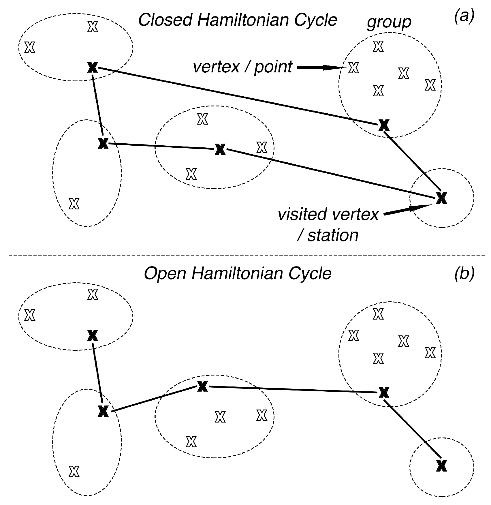
Figure 1a represents one possible closed Hamiltonian cycle, also known as g-tour, that visits exactly one vertex from each group before returning to the starting vertex. In
Figure 1b, the cycle is open as the start and end groups are discrete.
A discussion on how the GTSP can be used as one versatile and elegant tool to model different classes of combinatorial optimization problems like the covering tour problem, the material flow system design, the post-box collection problem, the stochastic vehicle routing problem, and the arc routing problem has been provided by [
11]. All these different use-cases show the importance of GTSP and E-GTSP in advanced GIS and city infrastructure planning and development. They have prime relevance in location-based problems, urban planning, postal routing problem, logistics problems, telecommunication problems, and railway track optimization problems. [
8,
12] have also discussed similar applications in detail.
Problem Encountered
In this study, the authors are primarily interested in the E-GTSP to TSP transformation, taking the location based services, vehicle routing and urban planning aspects into account. It should be noted that there already exists a large variety of exact and heuristic methods to solve a TSP [
13,
14,
15] like the state-of-the-art Lin–Kernighan–Helsgaun TSP solver [
9]. Since the underlying model represents an urban street setup, the authors have tried to think of this transformation from a spatial perspective. Five different possible search algorithms, motivated by the nearest neighbour search model [
16] and Voronoi model [
17], are suggested and tested on a real-world OpenStreetMap (OSM) street-network dataset to find the optimal search criterion for fast E-GTSP to TSP transformation. The idea is an extension of the authors’ previous work [
18]. This conversion is especially important for cases where the network or graph or cost-matrix of an urban street-network is generated on the fly (cases where cost is a function of time, like function of traffic congestion on the road). Different group-counts (i.e.,
) are employed to test all proposed algorithms for different complexity levels. Generated results are presented in graphical form and discussed in depth in the Results and Discussion section,
Section 5.
To the best of authors’ knowledge, this kind of spatial transformation of a given E-GTSP to TSP is the first of its kind and no related work is available in peer-reviewed literature online. It is believed that this study will further open research paradigms to improve existing search algorithms or to derive a better one for complex urban development and navigation problems. In the following sections, the proposed search algorithms are explained and tested on OSM derived road network data-set. Finally, a commentary on the results is provided in the Conclusions section.
2. Transformation of the E-GTSP to TSP
The GTSP was first introduced by [
4,
5,
6] through a record balancing problem that was aroused in the computer design. It is one of the few optimization problems that has extensively been studied in the past [
8,
19]. Researchers [
8,
20,
21,
22,
23,
24] have attempted to transform this into some efficient TSPs by exploiting the dynamic programming techniques [
25,
26], disintegrating a complex problem into a few simpler sub-problems). The shortcoming of this transformation, however, is that it dramatically increases the dimension of the problem, i.e., the dimension of the matrix representing the GTSP, thereby affecting the time and space consumption. Therefore, although theoretically it is possible to solve a given GTSP by converting it into corresponding TSP, the new increased problem size makes it computationally expensive to solve.
An E-GTSP solution of a vehicle-routing model is dependent upon the following two decisions in written order:
- 1
Selection of a subset of vertices (), also termed as stations, such that and for all . Note that .
- 2
Calculation of the minimum-cost Hamiltonian cycle in subgraph .
Since in our E-GTSP model the start and end vertices are different, the calculated g-tour is going to be an open one (
Figure 1b). Presented search algorithms do not increase the size of the problem by increasing the number of vertices or edges. Considering a vertex’s spatial distribution with respect to the start and end vertex, it is easier to filter-out distant and possibly sub-optimal vertices from each group. In this article,
points represent all possible vertices of
V including the start and end vertex,
group represents each set of vertex from
V exhibiting one particular attribute, and
station represents all selected points from each group (
Figure 1).
Points could be assumed as all supermarket, bank, etc. locations within a city,
group could be assumed as a set of certain attribute like
group of supermarket,
group of bank, etc., and
station could be assumed as those supermarket, bank, etc. locations that users should visit for least costly routes.
4. Study Area and Data-Set Used
In order to test all five proposed search algorithms, a real-world OSM street-network dataset is used. Fifteen cities belonging to the five different fractal dimension (frac-D) bins are selected for analysis out of the total 210 number of cities worldwide [
28] (
Figure 3). An increasing frac-D of an urban set-up represents its increasing road density, with 1D representing regions with only one road segment and 2D representing regions completely filled-up with road segments. Bin size in
Figure 3 has intentionally been kept small, i.e., 0.1, for finer fractally resolved classes. The Fractal Dimension Calculator is used to calculate the dimension of a city [
29].
Table 1 contains all analyzed cities, sorted with increasing value of frac-D, along with corresponding decisive attributes derived from the OSM vector dataset.
OSM dataset is downloaded from its Overpass API [
30] covering the bounding box of each selected city [
31]. All 105 start–end pairs are selected on the basis of the most visited locations by people, i.e., business center, tourist spot, and residential area. Five different groups of points representing bank, supermarket, cafe, pharmacy, and petrol-pump are taken from the OSM dataset to picture a near real-world E-GTSP routing instance. In total, only five such groups are selected from the OSM dataset for this study in order not to increase the brute-force processing time to find the optimal route. The whole processing is done in Python language. Instead of using the sample instances from existing GTSP libraries, like the GTSPLIB [
32], the authors have created their own E-GTSP instances from downloaded OSM vector data. This provides an opportunity to test the presented algorithms on specific urban planning and navigation scenarios. The authors have also provided the data/meta-data of all tested instances along with an optimal
set to encourage other researchers to carry out similar studies on OSM [
33]. Five E-GTSP instances with different
values are used for each selected city in order to run the discussed algorithms for various complexities. Key observations of the best algorithm and its behavior are discussed in
Section 5.
5. Results and Discussion
In order to test the five proposed search algorithms above for efficient E-GTSP to TSP transformation, 15 cities are selected based on their different level of street-network patterns and density (quantified by frac-D,
Table 1), for which the data was obtained from the OSM API. For each city, five different instances, i.e.,
, modeling various levels of E-GTSP complexity, are created and tested.
Figure 4a is a 3D-plot between the different search algorithms used, the different numbers of stations to be visited, i.e.,
, and the different types of street-networks. Here, each colored circle represents the average fractional error (average of the fractional errors coming out from all 105 analyzed start–end pairs) in the E-GTSP route-length estimated with respect to the optimal route (by brute-force). There are, in total, 375 (15 cities × 5 group-counts × 5 algorithms) colored circles, with black circles representing errors of more than 20%. It is clear that, irrespective of the choice of a given search algorithm, the percentage error in route length increases with higher
instances (marked by a big white arrow
Figure 4a). It is an expected behavior in a combinatorial optimization problem.
Figure 4b represents five graphs between different search algorithms and different type of street-networks, belonging to different
values. Black-boxes represent the lowest fractional error for that row. It can be seen that, for lower
values, the D-Search algorithm gives the lowest percentage error for the most number of cities, irrespective of their frac-Ds. However, this performance drifts away towards the R-Search algorithm for higher group-counts. It is an interesting observation that suggests that, for complex E-GTSP scenarios, it is better to select the optimal points that are radially close with respect to the start and end points. Another important observation is that, in spite of being hybrid, the performance of RE-Search and RD-Search was quite low. It should be noted that high computational complexity does not always mean better precision. Quantitatively, D-Search is the best one for all analyzed instances. However, it is important to understand how different algorithms have performed qualitatively (
Figure 5).
Figure 5a contains five different plots displaying the average fractional error for each city on the
y-axis, ordered according to
Table 1, for different
. Each colored circle represents one distinct search algorithm. In order to make the plots comparable, the red (D-Search) and green (R-Search) circles are connected. It can be seen that, for
the red line is almost always below the green one (
Figure 5a), showing its out-performance. However, for a higher
count, this observation is reversed. We have also already mentioned this observation in
Figure 4b.
Figure 5a allows us to compare them absolutely.
Figure 5b is a summation of the average fractional errors for all
instances for each city. It is clear that the green line lies below the red one for most of the cities. This makes R-Search, accuracy-wise, the best possible overall search-algorithm for any given E-GTSP to TSP transformation, particularly for urban planning and navigation use-cases. In vehicle routing problems, absolute route length acts as one vital attribute for any route selection process and, therefore, the R-Search approach should be considered. Figure 9 gives the percentage route-length error for different search-algorithms. R-Search gives the lowest average error of 8.8% when tested on a real-world dataset. It would be interesting to compare the performance of it with other approaches that are developed by [
25,
26] on a similar data-set.
Figure 6 gives one possible explanation of the performance of R-Search for higher
instances. The grey area is the proximity region of a given start–end points pair, while the white area is the region outside it. D-Search is quite efficient in selecting points lying close to the underlying Dijskstra route. Since this route terminates at the start–end points, points that lie behind them (white region,
Figure 6) do not get considered for stage 2 (
decision 1) (
Figure 2). On the other hand, R-Search remains unbiased towards points for their regions (white/grey) (
Figure 2). Although this leads to the total
number of TSP routes, the R-Search approach is better for white-regioned points. The
y-axis in
Figure 6 represents the average fraction of the total number of optimal stations for each
instance for white and grey regions. It should be noted that the number of optimal stations that fall within the grey-area gets lower with increase in complexity (
). This shows that, with increase in the number of group-counts, the more and more optimal stations come out from the white-region. This makes the performance of R-Search better. This is an interesting observation, which shows that different features/building functions in an urban city generally spread-out homogeneously. A continuous drop of the curve in
Figure 6 right helps us generalize the performance of R-Search for complex instances too.
In order to observe the D-Search and R-Search performance for increasing start–end points’ separation, a plot is generated between their estimated route length and optimal length (
Figure 7). The graph represents all 105 tested routes from all 15 cities for different complexities. The key observation here is the fanning-out behavior of all data points with increase in optimal route length. As one increases the best route length, the estimated value by both the algorithms gets farther away from the mean-line (solid) (
Figure 7). Although only the
scenario is presented here, a similar observation has been done for other instances too. This behavior is expected, as almost all routing algorithms get error-prone for distant start–end point pairs. Furthermore, in a given city’s road-network, the optimal route length of a complex E-GTSP instance might reach the order of a few couple of tens of kilometers. This shows the necessity to find the best possible solution in a timely fashion of a given TSP problem, as it will directly affect the time and money of the user.
Finally, a plot between the start–end points’ separation and their optimal route length value for different instances are created (
Figure 8). Instead of plotting the individual data-points on a graph, the authors have sketched their regions with differently styled lines for better visualization and explanation. With increase in the complexity of an instance (
) for a given city’s E-GTSP model, Brussels (Belgium) in this case, corresponding polygons drift away (marked by a solid arrow) from the mean-line towards some higher
y-value. On the right side of
Figure 8, there are two plots showing the slope of the trendline and
value with respect to the
. The trendline here belongs to each data-set that is sketched by the polygon. Each curve exemplifies one city model in
Figure 8. Decreasing slope of the trendline with increasing complexity shows the saturation of optimal route length value. It means that, for larger group-counts for the given E-GTSP model, the optimal route length becomes more independent from its start–end point geo-location. This observation is quite novel and shows that once an optimal route length of a given start–end pair for a complex instance is calculated, it could be extrapolated for other pairs too. Similar to the trendline, its
value also decreases with complexity. Furthermore, the decreased
value shows the complex street-networks of real-world cities. For complex instances, therefore, an amalgamation with heuristic approaches is advised, which is also necessary because a new route estimation for each scenario every time is computationally expensive.
6. Conclusions
The E-GTSP, which is an extension of the famous TSP, is proven by researchers to model a more realistic real-life combinatorial optimization problem, where the task is to find a close/open Hamiltonian cycle that visits exactly one vertex from each group in a given city. A recommended approach to solve this involves its reduction to the corresponding TSP before solving it to optimality. However, this transformation increases the dimension of the problem, thus making it computationally exhaustive (consuming time and RAM space) to solve for cases where the cost is a function of time. In this study, the authors have presented five different search algorithms for an E-GTSP to TSP transformation that operate spatially. They do not increase the count of the vertices or edges at any stage. They are tested on 15 selected cities, taken from the OSM dataset and classified into different road-networks, with five different instances each.
It is observed that, with increase in the complexity of a problem, all algorithms become erroneous, thereby making longer routes independent of the city’s street-pattern (
Figure 4a). For
instances, the D-Search is better among all discussed approaches; however, as one increases the value of
, i.e., instance complexity, R-Search gets better (
Figure 4b).
Figure 5b and
Figure 9 further support this observation by showing the minimum route-length value for R-Search. The performance of R-Search in this study could be attributed to its ability to consider stations belonging to regions lying outside the start–end proximity region (
Figure 6). It has also been observed that with increase in the optimal route length, its corresponding length error from D-Search or R-Search also gets bigger irrespective of the complexity of the instance (
Figure 7). One final observation, which proves the convoluted road networks of cities worldwide, is done in
Figure 8, where a deviation of data points away from the mean value line towards some saturation value is observed. It shows that, for a higher number of groups, i.e., increased complexity, the optimal route length of different start–end pairs becomes almost similar in value irrespective of their spatial separation.
This study, thus, brings forth a search criterion of point/vertex selection from each group for an E-GTSP to TSP transformation by testing many real-road networks. This search criterion, i.e., R-Search, considers the radial/spatial spread of points from each group with respect to the start and end point for the best possible selection. Readers can download the used dataset/meta-data from [
33]. A few other observations have also been documented regarding urban networks, which is believed to be helpful for urban planners.
Future research might involve the comparison of the R-Search criterion with other algorithms, like the state-of-the-art Lin–Kernighan–Helsgaun TSP solver, for E-GTSP to TSP conversion. Additional work might involve the development of a heuristic-R-Search (argued in this study) or ANN-R-Search algorithm. It is believed that this study will help geospatial and urban developers to solve location based problems that can be modelled into GTSP or E-GTSP by taking the spatial spread of points of interest into account.


