Simulation Experiment and Mathematical Model of Liquid Carrying in the Entire Wellbore of Shale Gas Horizontal Wells

Abstract

Shale gas is mostly produced using horizontal wells, since shale gas reservoirs have low porosity and permeability. It is challenging to predict a horizontal well’s critical liquid-carrying gas flow rate because horizontal wells have more complicated well structures and gas–liquid two-phase pipe flows than vertical wells. In addition, there are significant differences between shale gas reservoirs and conventional natural gas reservoirs as well as dynamic changes in the liquid production rate. The majority of critical liquid-carrying models currently in use in engineering are based on the force analysis of droplets in the gas stream or liquid film on the pipe wall in annular-mist flow in the vertical wellbore. However, they do not take into account the impact of changes to the entire wellbore structure and dynamic changes in the liquid production rate on gas–liquid two-phase flow patterns and liquid carrying in the wellbore. In order to perform the critical gas velocity test for liquid carrying in the entire wellbore of horizontal wells, a visual liquid-carrying simulation experimental device for the entire wellbore of horizontal wells and a high-speed camera were used in this study. The onset of liquid accumulation was analyzed comprehensively according to the overall increase of the wellbore liquid and the change of the system pressure. A modified K–H wave theory liquid-carrying model was developed by taking into account the impacts of liquid production rate and well inclination angle based on the experimental data, the K–H wave theory, the cross-section actual gas velocity, and the angle correction correlation formula. The improved liquid-carrying model is in good accordance with the test findings, according to the experimental results. In Shunan Gas Mine, Sichuan, China, there are eight deep shale gas wells, which produced a total of 25 sets of tests. The modified model was used to forecast and diagnose the liquid-carrying capacity in the entire wellbore of these wells. The diagnosis results are in good agreement with the actual production situation, and the coincidence rate is 92%.

1. Introduction

In the process of extracting shale gas, a significant amount of fracturing fluid is used, which leads to shale gas wells producing fluid for an extended period of time. The liquid builds up at the bottom of the well to create liquid accumulation if the gas velocity or formation energy are too low [1,2]. On the contrary, if the gas velocity or pressure is sufficient, the liquid flowing into the bottom of the well from the formation will be lifted out of the wellhead; that is, the liquid-carrying condition is satisfied, and the gas well has normal and stable production. Unfortunately, the most common problem in natural gas production is fluid accumulation at the bottom of the well. Although much research has been carried out with regard to this problem, studies are mainly aimed at conventional gas reservoirs or vertical wells. A number of models have been created to forecast the critical liquid-carrying gas flow rate in gas wells based on the Turner droplet model [1,2,3,4,5,6,7,8,9,10]. However, they are rarely targeted at shale gas wells.

For horizontal gas wells, scholars have proposed an angle-modified model based on the Turner droplet model. For example, Belfroid et al. [11] experimentally studied the liquid carrying of gas–liquid two-phase flow at different inclination angles, considered the difference in pipe diameter, and added the inclination correction term to the Turner prediction model through the Fiedler [12] shape function. Veeken et al. [13] analyzed the sensitivity of different gas well parameters and critical flow rate, and the Turner model was modified according to the modeling results of steady-state and transient multiphase flows. Li et al. [14] conducted three-dimensional fitting of superficial liquid velocity and inclined angles according to the experimental data, obtaining an empirical formula applicable to angles of 0–90° and a superficial liquid velocity range of 0.01–0.1 m/s. Zhou et al. [15] established a full-hole critical liquid-carrying flow rate model of a shale gas well through analyzing droplet dynamics and energy and by comprehensively considering the droplet energy loss caused by the liquid production rate, droplet deformation, and build-up rate change in the wellbore. In addition to these studies, there are liquid-carrying models based on liquid film inversion as the onset of liquid accumulation [11,12,13,14,15,16,17,18,19] as well as liquid-carrying models based on energy analysis [10,19,20,21]. While the premise of such models must satisfy the conditions of annular-mist flow, the critical liquid-carrying gas velocity or gas flow rate obtained does not satisfy the conditions of annular-mist flow or is inconsistent with the actual gas–liquid two-phase pipe flow regime of gas wells under normal production [4,5,6,7,8,9,22,23,24,25,26]. At the same time, the above models do not consider the influence of the change of the full wellbore structure and the dynamic change of fluid production flow rate on the gas–liquid two-phase pipe flow regime and liquid carrying of shale gas horizontal wells.

The commonly used liquid-carrying models in gas wells are not related to liquid production flow rate. Under the condition of high gas–liquid ratio, when the annular-mist flow is achieved, these models may be reasonable; however, for deep shale gas wells, the liquid production flow rate is large, and flow conditions usually cannot reach the annular-mist flow pattern, then they are not suitable for shale gas horizontal wells. Therefore, we carried out critical liquid-carrying gas flow velocity tests for the full wellbore of shale gas horizontal wells and determined the critical liquid-carrying state according to the balance of inlet and outflow liquid flow and the stability of pressure, rather than solely based on droplet fall or liquid film reflux. A shale gas liquid-carrying model was created by combining experimental data with the Kelvin–Helmholtz (K–H) unstable gas–liquid two-phase flow theory [27,28] and taking well inclination angle and liquid production rate into account.

2. Experimental Facility and Method

In order to carry out liquid-carrying simulation experiments in the entire wellbore of shale gas horizontal wells, this work developed a liquid-carrying simulation experimental setup of the whole wellbore of a horizontal well. The total pipe length was about 16.5 m. The main test pipe was made of transparent PVC pipe, which can withstand a pressure of 1.0 MPa, with 6 sensors installed. The measuring points were spaced 2 m apart in the horizontal segment, 0.75 m apart in the inclined segment, and 1 m apart in the vertical segment. In addition, a quick-closing valve (manual valve) was configured in the inclined segment to test the liquid holdup. The experimental schematic diagram and setup are shown in Figure 1a,b.

In the experiment, air and water were used as the fluid medium. The air was pressurized by the compressor and measured by the flowmeter before being injected into the test pipeline from the inlet, and the water was injected from the inlet through a metering pump. The outlet throttle valve (manual valve) was used to regulate the system’s pressure. The inclined segment was connected with the horizontal and vertical segments by a pressure-resistant transparent hose, which was convenient for adjusting the angle of the inclined segment. The experimental temperature was normal temperature (about 25 °C during the test). During the experiment, prior to injecting any liquid or gas into the experimental pipeline, the gas and liquid flow rates were measured; at the same time, the outlet liquid volume was recorded with a water tank. The liquid-carrying state of each segment and the whole wellbore was judged by observing the gas–liquid two-phase flow regime and liquid backfall in horizontal, inclined, and vertical segments as well as the liquid volume in the water tank. If in a critical state, the critical liquid-carrying gas velocity could be calculated using the pressure, pressure difference, pipe diameter, and gas flow rate.

3. Experimental Results and Analysis

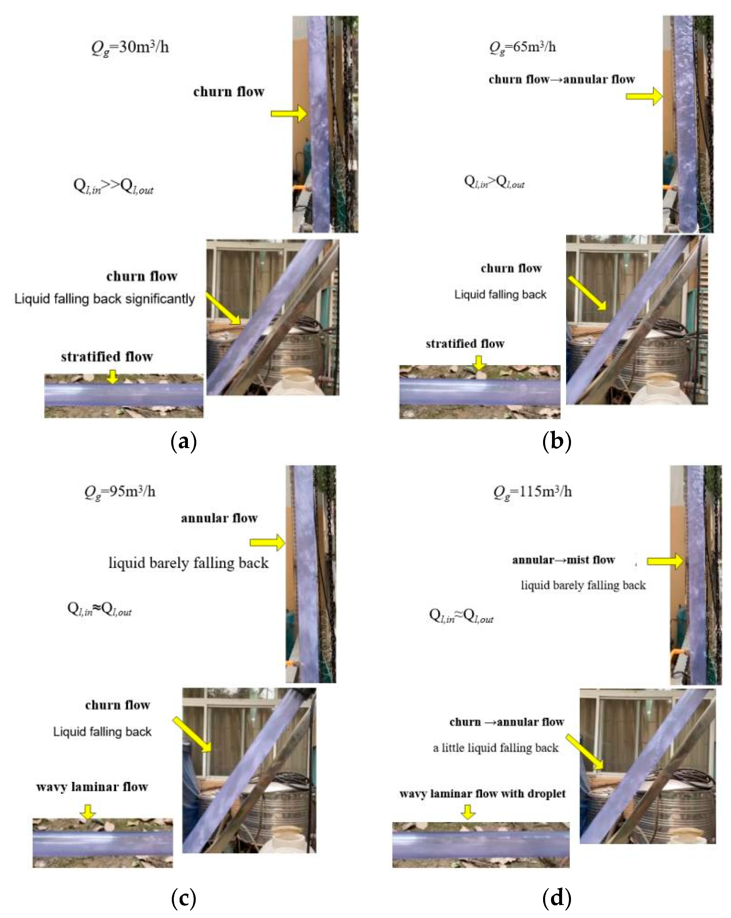
3.1. Experimental Phenomena

The experimental test inclination angles comprised 0°, 15°, 30°, 45°, 60°, 80°, and 90° (angles in the horizontal direction), where 0° and 90° were tested in the horizontal observation segment and vertical observation segment, respectively, and the remainder of the angles were tested by adjusting the inclination segment angle. Figure 2 shows the change of the gas–liquid two-phase flow regime of the whole wellbore, liquid flow characteristics of each segment, and Q_L,in and Q_L,out of the system when the angle of the inclined segment is 45°, the system pressure is 100 kPa, and the gas flow Q_g is 30 m³/h, 65 m³/h, 95 m³/h, and 115 m³/h.

The liquid flow in the horizontal segment of Figure 2a depends mostly on the liquid supply when the gas flow rate is 30 m³/h (the liquid flow rate is 0 or 0.1 m³/h). If there is no liquid supply, very little liquid flows out of the outlet, and almost no liquid flows in the horizontal segments. Both the inclined and vertical portions clearly exhibit liquid reflux, and the amount of liquid entering the system is significantly greater than the amount of liquid leaving it. The system pressure rises as the overall amount of wellbore liquid grows, and it becomes clear that liquid is accumulating in the pipes.

The liquid in the horizontal segment can flow under the action of gas when the gas flow rate is 65 m³/h (liquid flow rate is 0 or 0.1 m³/h); the inclined segment is characterized by churn flow, and liquid reflux is visible. The vertical segment displays the characteristics of gas–liquid two-phase churn flow–annular flow, with a small amount of liquid falling back. The amount of liquid flowing into the system is greater than its outflow (in the absence of a steady supply of liquid, some of the liquid stored in the pipe flows out of the outlet), and the liquid accumulates in the pipe.

The horizontal segment displays a wavy laminar flow regime when the gas flow rate is 95 m³/h (the liquid flow rate is 0 or 0.1 m³/h), and the liquid can flow under the action of the gas (independent of liquid supply); the liquid exhibits a certain fallback, and the inclined segment exhibits churn flow characteristics. The liquid practically does not fall back in the vertical segment, which demonstrates the properties of annular-mist flow. There is essentially no liquid buildup in the pipe, since the system’s liquid input and outflow are roughly equal.

A tiny number of liquid water droplets at the top of the pipe travel and scatter down the pipe wall when the gas flow rate is 115 m³/h (the liquid flow rate is 0 or 0.1 m³/h); the horizontal segment displays a wavy laminar flow regime, and a small number of liquid droplets are transported in the gas flow center. The liquid practically does not fall back in the inclined segment, which exhibits churn flow and annular flow features. The liquid does not fall back in the vertical segment, which displays the properties of annular-mist flow. There is no liquid buildup in the pipe, since the system’s liquid input and outflow are almost equal.

The wavy laminar flow, intermittent flow, and other flow regimes arise in the horizontal segment with an increase in liquid flow rate (0, 0.1–0.5 m³/h), whereas slug flow, churn flow, and other flow regimes appear in the inclined and vertical segments. The inflow liquid volume of the system can eventually be almost equal to the outflow liquid volume without the features of liquid buildup, even if slug flow, churn flow, and other flow regimes (including at the wellhead) appear in the pipe.

Under the same or similar pressure and temperature conditions, the analysis in Figure 2 shows that liquid retention is more likely in the inclined pipe segments, but the onset of liquid accumulation should not be solely determined by the presence of liquid fallback in a particular segment (only at extremely high gas flow rates does liquid reflux not occur; liquid reflux can be seen under common flow regimes, such as slug flow, churn flow, and annular flow). The overall amount of wellbore fluid and changes in system pressure should be considered when determining the onset of the liquid accumulation. The liquid fallback should be taken into account as the criterion for the onset of liquid accumulation if it influences the rise in system pressure; otherwise, the onset of liquid accumulation should be judged according to whether the total wellbore liquid volume increases or not.

3.2. Test Results and Analysis of Critical Liquid-Carrying Gas Velocity

According to the above method of judging liquid accumulation, when the outlet pressure of the system is approximately 100 kPa under the condition of low liquid flow rate, the critical liquid-carrying gas velocity of different well inclination angles is tested, as shown in

Table 1. Critical liquid-carrying velocity (v_cr) at different well inclination angles (θ).

θ, o	90	80	60	45	30	15	0
vcr, m/s	8.57	10.15	11.37	12.38	12.4	10.89	6.22

. It can be seen from the test that the system pressure increases and the liquid-carrying velocity decreases. The maximum liquid-carrying gas velocity occurs between a 30° and 45° inclination angle (it is not possible to judge the location of liquid accumulation simply by the angle of inclination because the flow conditions at different incline depths of the actual wellbore are quite different), and the minimum occurs at a 0° inclination angle (i.e., horizontal). Meanwhile, the test results show that the larger the liquid flow rate, the lower the critical liquid-carrying flow rate.

4. Evaluation of Wellbore Liquid-Carrying Model

According to the experimental results of liquid carrying in the entire wellbore of horizontal gas wells, the Turner model [1], Li Min model [3,4], Belfroid model [11], and K–H wave theory model [27,28] were used to predict the critical liquid-carrying gas velocity (using pressure of 100 kPa and air and water as medium) under different well deviation angle conditions, as shown in

Table 2. Comparison of liquid-carrying models.

θ, °	Test Critical Liquid-Carrying Velocity, m/s	Turner Model, m/s	Li Min Model, m/s	Belfroid Model, m/s	K–H Wave Theory Model, m/s
90	8.57	16.45	6.23	16.47	0
80	10.15	16.45	6.23	19.36	8.06
60	11.37	16.45	6.23	22.05	10.50
45	12.38	16.45	6.23	21.99	11.45
30	12.40	16.45	6.23	20.20	12.04
15	10.89	16.45	6.23	16.14	12.38
0	6.26	16.45	6.23	/	12.48

.

As shown in Table 2, the Turner and Li Min models do not take into account the impact of well inclination angle, and their critical liquid-carrying gas velocity does not consider angle, which contradicts the test results. When the Belfroid model and the K–H wave theory model are compared to the test findings, the trend of the Belfroid model is largely compatible with the test results, although its value is noticeably larger. The K–H wave theory model’s predicted value is close to the observed value; however, the trend is not consistent. The average absolute error of the Belfroid model is 77.63%, while the average absolute error of the K–H wave theory model is 35.98%, according to the findings of the error analysis.

5. Model Modification and Verification

From the comparison between the theoretical K–H wave theory model and the test results, we find that the values are close, but the trends are quite different, especially around the inclination angles of 0° and 90°. Therefore, the angle correction item of the Belfroid model is used for reference, and the K–H wave theory model is modified as follows.

The critical velocity [27,28] of K–H unstable flow theory is

$$v_{cr,sg}=2\sqrt{2}{\left(\frac{g\sigma \cos \theta {\rho }_l}{{\rho }_g^2}\right)}^{0.25}$$

(1)

According to the angle correction item of the Belfroid model [11], the above formula is modified to

$$v_{cr,sg}=2\sqrt{2}{\left(\frac{g\sigma \sin \left(1.7\theta \right){\rho }_l}{{\rho }_g^2}\right)}^{0.25}$$

(2)

Under the condition of annular-mist flow, the turbulence degree is high, the liquid holdup is low, the gas flow velocity is approximately equal to the superficial gas flow velocity, v_sg, and the effect of the liquid production rate can be ignored. However, for other gas–liquid two-phase pipe flow regimes, when the gas–liquid flows through the tubing segment at the same time, the liquid occupies part of the cross section of tubing. The real gas flow velocity is higher than the superficial gas flow velocity, and it is easier to carry liquid. Therefore, the real gas velocity correction is adopted, and the correction coefficient β_L is as follows:

From

$$v_g=\frac{v_{sg}}{1-H_L}$$

we obtain

$${\beta }_L=\frac{v_{sg}}{v_g}=1-H_L$$

(3)

where v_g is the real gas flow velocity, m/s; v_sg is the superficial gas flow velocity, m/s; and H_L is calculated using the following formula [29]:

$$H_L=1-\frac{v_{sg}}{1.208\left(v_{sg}+v_{sl}\right)+1.41{\left[\frac{g\sigma \left({\rho }_l-{\rho }_g\right)}{{\rho }_l^2}\right]}^{0.25}\sqrt{\sin \theta }}$$

where g is the acceleration of gravity, 9.81 m/s²; v_sl is the superficial liquid flow velocity, m/s; σ is the surface tension, N/m; and ρ_g and ρ_l are the gas and liquid density, kg/m³, respectively.

In the above formula, if H_L is less than the no-slip holdup level, the holdup H_L should be taken as the no-slip holdup level.

By combining Equations (2) and (3), the liquid-carrying model modified by K–H wave theory and considering the effect of liquid holdup H_L (the liquid production rate will affect the liquid holdup, which will indirectly affect the critical gas flow velocity) and well incline angle is obtained:

$$v_{cr}=v_{cr,sg}\left(1-H_L\right)=2\sqrt{2}{\left(\frac{g\sigma \sin \left(1.7\theta \right){\rho }_l}{{\rho }_g^2}\right)}^{0.25}\left(1-H_L\right)$$

(4)

In the above formula, θ is the included angle between the wellbore and the horizontal direction, and the applicable angle range is 5° ≤ θ ≤ 90°. When θ = 0°, calculations are made according to the following formula; when 0° < θ < 5°, Equation (4) and the following equations are used to calculate using linear interpolation.

$$v_{cr}=\sqrt{2} {\left(\frac{g\sigma {\rho }_l}{{\rho }_g^2}\right)}^{0.25}\left(1-H_L\right)$$

(5)

The calculation results of the K–H wave theory liquid-carrying model after modification are shown in

Table 3. Error analysis of the modified K–H wave theory model at different well inclination angles (θ).

θ, °	Test Critical Liquid-Carrying Velocity, m/s	K–H Wave Theory Modified Model
		Critical Velocity, m/s	Absolute Percentage Error, %
90	8.57	9.84	14.82
80	10.15	10.93	7.68
60	11.37	11.92	4.84
45	12.38	12.15	1.86
30	12.40	11.62	6.29
15	10.89	10.10	7.25
0	6.26	6.18	1.28
the average absolute error, %			6.29

. The maximum error of the K–H wave theory model after modification is 14.82%, and the average absolute error is 6.29%, which significantly improves the accuracy compared with that before modification.

6. Application and Discussion

Verification and evaluation were carried out on eight typical deep shale gas test wells totaling 25 sets of tests from 2020 to 2023 in Shunan Gas Mine, Sichuan, China. These tests covered the casing production stages of each well as well as the running tubing production stage. The production casing was 139.7 mm (wall thickness 12.7 mm, inner diameter 114.3 mm). After casing production for a period of time, 70 mm (ID 62 mm) tubing was run in Y-H1 and Y-H2 wells, and 60.3 mm (ID 50.6 mm) tubing was run in the other wells. The running depth of tubing was near point A, and the length of the horizontal segment was between 1800 m and 2300 m.

According to gas well production tests and production history data, the production status of each gas well was obtained, and the results are shown in

Table 4. Production test and production status of gas wells.

No.	Well No.	Test Date	pwh, MPa	Qg, 104 m3/d	Ql, m3/d	Production String	Status
1	Y-H1	3 March 2022	46.39	21.01	170.4	casing	Unloaded
2	Y-H1	1 October 2022	8.88	5.48	15.5	casing	Loaded
3	Y-H1	14 November 2022	11.59	6.9	15.47	Tubing 4200 m	Unloaded
4	Y-H2	19 September 2020	13.52	5.83	47	casing	Loaded
5	Y-H2	30 September 2020	26.53	7.28	33	Tubing 4200 m	Unloaded
6	Y-H2	7 January 2022	4.14	2.58	12	Tubing 4200 m	Loaded
7	Y-H3	21 May 2021	39.71	9.92	110	casing	Unloaded
8	Y-H3	29 December 2021	17.24	5.91	72	casing	Loaded
9	Y-H3	30 July 2022	5.73	2.86	20	Tubing 4056 m	Unloaded
10	L-H4	30 September 2020	16.42	12.37	70	casing	Unloaded
11	L-H4	31 October 2020	8.25	5.32	40	casing	Loaded
12	L-H4	20 November 2020	6.48	7.3	19	Tubing 4100 m	Unloaded
13	L-H4	5 September 2021	4.2	5.09	12	Tubing 4100 m	Unloaded
14	L-H4	17 January 2023	3	2.41	1	Tubing 4100 m	Loaded
15	L-H5	20 October 2021	20.89	12.05	52	casing	Impending
16	L-H5	18 November 2021	17.84	12.64	42	Tubing 4467 m	Unloaded
17	L-H5	21 March 2023	5.33	3.97	7	Tubing 4467 m	Unloaded
18	W-H6	23 August 2021	14.2	3.39	4	casing	Loaded
19	W-H6	14 September 2021	8.1	5.34	28	Tubing 3330 m	Unloaded
20	W-H6	21 February 2023	2.37	1.21	4	Tubing 3330 m	Loaded
21	Y-H7	14 September 2021	17.9	10.6	11.34	casing	Loaded
22	Y-H7	12 October 2021	21.02	12.65	22	Tubing 4135 m	Unloaded
23	Y-H8	19 May 2022	10.24	4.34	67.2	casing	Loaded
24	Y-H8	10 June 2022	9.22	5.1713	38	Tubing 3988 m	Unloaded
25	Y-H8	14 January 2023	4.28	5.58	45	Tubing 3988 m	Unloaded

.

According to the liquid-carrying model established in this study, liquid accumulation diagnosis and analysis were carried out on deep shale gas wells (25 sets of tests, including the production conditions of each well at different production times). The results are shown in

Table 5. Prediction and diagnosis of liquid loading.

No.	Well No.	Status	The New Improved Model				Belfroid Model
			Qg,crit 104 m3/d	Depth and Angle m@°	Results	Wellhead Qg,crit 104 m3/d	Qg,crit 104 m3/d	Results
1	Y-H1	Unloaded	11.99	[email protected]°	Unloaded	10.83	26.55	Loaded
2	Y-H1	Loaded	9.53	[email protected]°	Loaded	7.7	19.28	Loaded
3	Y-H1	Unloaded	4.42	[email protected]°	Unloaded	2.83	14.58	Loaded
4	Y-H2	Loaded	10.28	[email protected]°	Loaded	7.97	23.04	Loaded
5	Y-H2	Unloaded	3.93	[email protected]°	Unloaded	3.48	7.77	Loaded
6	Y-H2	Loaded	2.57	[email protected]°	Impending	1.73	4.98	Loaded
7	Y-H3	Unloaded	11.47	[email protected]°	Loaded	9.35	28.71	Loaded
8	Y-H3	Loaded	10.19	[email protected]°	Loaded	7.7	25.39	Loaded
9	Y-H3	Unloaded	1.98	[email protected]°	Unloaded	1.32	3.93	Loaded
10	L-H4	Unloaded	11.73	[email protected]°	Unloaded	9.28	24.14	Loaded
11	L-H4	Loaded	9.30	[email protected]°	Loaded	7.02	20.00	Loaded
12	L-H4	Unloaded	4.32	[email protected]°	Unloaded	1.43	10.77	Loaded
13	L-H4	Unloaded	3.74	[email protected]°	Unloaded	1.18	9.35	Loaded
14	L-H4	Loaded	2.738	[email protected]°	Loaded	1.04	6.84	Loaded
15	L-H5	Impending	12.32	[email protected]°	Loaded	10.27	24.77	Loaded
16	L-H5	Unloaded	8.66	[email protected]°	Unloaded	2.09	10.58	Unloaded
17	L-H5	Unloaded	3.07	[email protected]°	Unloaded	1.35	9.23	Loaded
18	W-H6	Loaded	10.21	3202m@46°	Loaded	8.12	23.09	Loaded
19	W-H6	Unloaded	4.57	[email protected]°	Unloaded	1.54	17.32	Loaded
20	W-H6	Loaded	2.71	[email protected]°	Loaded	0.9	10.73	Loaded
21	Y-H7	Loaded	12.35	[email protected]°	Loaded	10.86	23.69	Loaded
22	Y-H7	Unloaded	5.03	[email protected]°	Unloaded	2.37	15.63	Loaded
23	Y-H8	Loaded	8.83	[email protected]°	Loaded	6.53	21.99	Loaded
24	Y-H8	Unloaded	4.09	[email protected]°	Unloaded	1.56	19.81	Loaded
25	Y-H8	Unloaded	1.97	[email protected]°	Unloaded	1.109	5.97	Loaded
Correct ratio					23/25 = 0.92	21/25 = 0.84		13/25 = 0.6

. The diagnosis results of the entire wellbore are basically consistent with the actual production conditions. Only Y-H3 with unloaded status (21 May 2021) and L-H5 with impending loaded status (20 October 2021) were incorrectly diagnosed as loaded status. The possible reason for this is that there are errors in the prediction of pressure gradient and liquid holdup, which lead to some deviations in the results. If the pressure distribution and liquid holdup can be accurately predicted, the results will be improved.

From the angle and depth of the wellbore where the maximum liquid-carrying gas flow rate is located, the location of the required maximum liquid-carrying gas flow rate cannot be determined simply using the range of the well inclination angle; this is mainly due to the large difference in flow conditions at the different well inclination depths. When the tubing depth does not reach the large deviated well segment (inclination angle < 20°), the maximum liquid-carrying gas flow rate may also appear in the large deviated well segment, as shown in the corresponding results of Nos. 17, 19, 20, etc., in Table 5.

According to the diagnosis of wellhead flow conditions, it is easy to wrongly diagnose the loaded gas wells as having unloaded status, which delays the time to take measures, as shown in Nos. 6, 14, 15, and 20 in Table 5. Meanwhile, the critical liquid-carrying flow rate predicted at the wellhead is smaller than that of the entire wellbore. It can be seen that judging the critical liquid-carrying flow rate or velocity of horizontal shale gas wells using wellhead conditions can lead to inaccuracies; these should be judged comprehensively using the flow conditions of the entire wellbore.

It is too conservative to predict the critical liquid-carrying gas flow rate of a shale gas well according to the angle correction model of the Belfroid and Turner types; the prediction of the critical liquid-carrying gas flow rate is generally too high. Therefore, it is easy to misdiagnose the unloaded liquid well as the loaded liquid well and take premature measures to increase production costs.

7. Conclusions

(1)

The horizontal well liquid-carrying simulation test along the whole wellbore revealed that the inclined pipe segment, which is the initial location of liquid accumulation in horizontal shale gas wells, is where liquid carrying in horizontal wells is most challenging. However, it is not sufficient to check only a particular segment for liquid fallback; the liquid fallback can be seen under common flow regimes such as slug flow, churn flow, and annular flow.

(2)

According to experimental tests, for the same flow conditions, the highest liquid carrying gas flow velocity occurs between a 30° and 45° inclination angle, and the minimum occurs at a 0° inclination angle (i.e., horizontal angle). However, as the flow characteristics of the real wellbore fluctuate significantly with different inclination depths, the position of the liquid loaded should not be determined purely by the inclination angle.

(3)

A modified K–H wave theory liquid-carrying model was established. The experimental results showed that the modified liquid-carrying model was in good agreement with the test results, and the coincidence rate was about 92%. The modified model was used to predict and diagnose the liquid carrying in the whole wellbore of eight typical deep shale gas wells. The results were consistent with the actual production situation. Considering only the liquid-carrying gas velocity in the gas well based on the wellhead conditions can lead to misjudgment; a comprehensive determination should be made according to the flow conditions in the whole wellbore.

(4)

The accuracy of the model can be better verified by considering the production state of each of the sample test wells as well as individual wells under loaded and unloaded liquid production states.

References

1. Turner, R.G.; Hubbard, M.G.; Dukler, A.E. Analysis and Prediction of Minimum Flow Rate for the Continuous Removal of Liquids from Gas Wells. JPT 1969, 21, 1475–1481. [Google Scholar]
2. Li, M. Coiled tubing of drainage gas recovery technology used in shale-gas downdip horizontal wells. Oil Drill. Prod. Technol. 2020, 42, 329–333. (In Chinese) [Google Scholar]
3. Coleman, S.B.; Clay, H.B.; Mccurdy, D.G.; Norris, L.H.I. A new look at predicting gas-well load-up. J. Pet. Technol. 1991, 43, 329–333. [Google Scholar]
4. Li, M.; Guo, P.; Tan, G. New Look on Removing Liquids from Gas Wells. Pet. Explor. Dev. 2001, 28, 125–126. [Google Scholar]
5. Li, M.; Sun, L.; Li, S. A New Gas Well Liquid Continuous Withdrawal Model. Nat. Gas Ind. 2001, 21, 61–63. [Google Scholar]
6. Wang, Y.; Liu, Q. A new method to calculate the minimum critical liquids carrying flow rate for gas wells. Pet. Geol. Oilfield Dev. Daqing 2007, 26, 82–85. [Google Scholar]
7. Wei, N.; Li, Y.; Li, Y.; Liu, A.; Liao, K.; Yu, X. Visual Experimental Research on Gas Well Liquid Loading. Drill. Prod. Technol. 2007, 30, 43–45. [Google Scholar]
8. Peng, C. Study on Critical Liquid-Carrying Flow Rate for Gas Well. Xinjiang Pet. Geol. 2010, 31, 72–74. [Google Scholar]
9. Wang, Z.; Li, Y. The mechanism of continuously removing liquids from gas wells. Acta Pet. Sin. 2012, 33, 681–686. [Google Scholar]
10. Zhou, D.-S.; Zhang, W.-P.; Li, J.-X.; Song, P.-J. Multi-droplet model of liquid unloading in natural gas wells. J. Hydrodyn. 2014, 29, 572–579. [Google Scholar]
11. Belfroid, S.; Schiferli, W.; Alberts, G.; Veeken, C.A.; Biezen, E. Predicting onset and dynamic behaviour of liquid loading gas well. In SPE Annual Technical Conference and Exhibition; Society of Petroleum Engineers: Denver, CO, USA, 2008. [Google Scholar] [CrossRef]
12. Fiedler, S.; Auracher, H. Experimental and theoretical investiga tion of reflux condensation in an inclined small diameter tube. Int. J. Heat Mass Transf. 2004, 47, 4031–4043. [Google Scholar]
13. Veeken, K.; Hu Bin Schiferli, W. Gas-well liquid-loading-field-data analysis and multiphase-flow modeling. SPE Prod. Oper. 2010, 25, 275–284. [Google Scholar]
14. Li, J.; Almudairs, F.; Zhang, H. Prediction of Critical Gas Velocity of Liquid Unloading for Entire Well Deviation. IPTC 2014, 12. [Google Scholar] [CrossRef]
15. Zhou, C.; He, Z.; Fu, D.; Luo, X.; Liu, H.; Sun, Z. Full-hole critical liquid carrying flow model of shale-gas horizontal well. Oil Drill. Prod. Technol. 2021, 43, 791–797. [Google Scholar]
16. Lei, D.; Du, Z.; Shan, G.; Tang, Y. Calculation method for critical flow rate of carrying liquid in horizontal gas well. Acta Pet. Sin. 2010, 31, 637–639. [Google Scholar]
17. Luo, S.; Kelkar, M.; Pereyra, E.; Sarica, C. A new comprehensive model for predicting liquid loading in gas wells. SPE Prod. Oper. 2014, 29, 337–349. [Google Scholar]
18. Fan, Y.; Pereyra, E.; Sarica, C. Onset of Liquid-Film Reversal In Upward-Inclined Pipes. SPE J. 2018, 10, 1630–1647. [Google Scholar]
19. Liu, Y.; Ai, X.; Luo, C.; Liu, F.; Wu, P. A new model for predicting critical gas velocity of liquid loading in horizontal well. J. Shenzhen Univ. Sci. Eng. 2018, 35, 551–557. [Google Scholar]
20. Wu, Z.; He, S. Determination of the critical liquid carrying flow rate at low gas liquid ratio. Pet. Explor. Dev. 2004, 31, 108–109. [Google Scholar]
21. Guo, B.; Ghalambor, A.; Xu, C. A systematic approach to predicting liquid loading in gas wells. SPE Prod. Oper. 2006, 21, 81–88. [Google Scholar]
22. Zhao, Z.J.; Liu, T.; Xu, J.; Zhu, J.; Yang, Y. Stable fluid-carrying capacity of gas wells. Nat. Gas Ind. 2015, 35, 59–63. [Google Scholar]
23. Wang, Q. Experimental Study on Gas-Liquid Flowig in the Wellbore of Horizontal Well; Southwest Petroleum University: Chengdu, China, 2014. [Google Scholar]
24. He, Y.; Li, Z.; Zhang, B.; Gao, F. Design optimization of critical liquid-carrying condition for deepwater gas well testing. Nat. Gas Ind. 2017, 37, 63–70. [Google Scholar]
25. Wang, R.; Ma, Y.; Dou, L.; Chen, J.; Zhang, N. Review of Critical Liquid Unloading Rate Models and Liquid Loading Models for Gas Well Producing Water. Sci. Technol. Eng. 2019, 19, 10–20. [Google Scholar]
26. Zhong, H.; Zheng, C.; Li, M.; Liu, T.; He, Y.; Li, Z. Transient Pressure and Temperature Analysis of a Deepwater Gas Well during a Blowout Test. Processes 2022, 10, 846. [Google Scholar] [CrossRef]
27. Hsieh, D.Y. Kelvin-Helmholtz stability and two-phase flow. Acta Math. Sci. 1989, 9, 189–197. [Google Scholar] [CrossRef]
28. Xiao, G. Theory and Experiment Research on the Liquid Continuous Removal of Horizontal Gas Well. J. Southwest Pet. Univ. 2010, 32, 122. [Google Scholar]
29. Kaya, A.S.; Sarica, C.; Brill, J.P. Mechanistic Modeling of Two-phase in Deviated Wells. SPE Prod. Facil. 2001, 16, 156–165. [Google Scholar] [CrossRef]
Figure 1. Schematic diagram and setup of horizontal well liquid-carrying simulation experiment. (a) Schematic diagram; (b) facility.
Processes 11 02339 g001
Figure 2. Flow characteristics of the whole wellbore with different gas flow rates. (a) (Qg = 30 m3/h). (b) (Qg = 65 m3/h). (c) (Qg = 95 m3/h). (d) (Qg = 115 m3/h).
Processes 11 02339 g002