
Drone-Based Measurement of the Size Distribution and Concentration of Marine Aerosols above the Great Barrier Reef

 , , and
Abstract
:1. Introduction

2. Materials and Methods
2.1. Sampling Methodology
2.2. Setup Hardware
2.3. Modelling Data and Analysis
3. Results
4. Discussion
5. Conclusions
Author Contributions
Funding
Data Availability Statement
Acknowledgments
Conflicts of Interest
References
- O’Dowd, C.D.; De Leeuw, G. Marine aerosol production: A review of the current knowledge. Philos. Trans. R. Soc. A Math. Phys. Eng. Sci. 2007, 365, 1753–1774. [Google Scholar] [CrossRef] [PubMed]
- Saltzman, E.S. Marine aerosols. Geophys. Monogr. Ser. 2009, 187, 17–35. [Google Scholar]
- Murphy, D.M.; Anderson, J.R.; Quinn, P.K.; McInnes, L.M.; Brechtel, F.J.; Kreidenweis, S.M.; Middlebrook, A.M.; Pósfai, M.; Thomson, D.S.; Buseck, P.R. Influence of sea-salt on aerosol radiative properties in the Southern Ocean marine boundary layer. Nature 1998, 392, 62–65. [Google Scholar] [CrossRef]
- Andreae, M.O.; Jones, C.D.; Cox, P.M. Strong present-day aerosol cooling implies a hot future. Nature 2005, 435, 1187–1190. [Google Scholar] [CrossRef] [PubMed]
- Jacobson, M.Z. Global direct radiative forcing due to multicomponent anthropogenic and natural aerosols. J. Geophys. Res. Atmos. 2001, 106, 1551–1568. [Google Scholar] [CrossRef]
- Quinn, P.K.; Coffman, D.J.; Johnson, J.E.; Upchurch, L.M.; Bates, T.S. Small fraction of marine cloud condensation nuclei made up of sea spray aerosol. Nat. Geosci. 2017, 10, 674–679. [Google Scholar] [CrossRef]
- Ayash, T.; Gong, S.; Jia, C.Q. Direct and Indirect Shortwave Radiative Effects of Sea Salt Aerosols. J. Clim. 2008, 21, 3207–3220. [Google Scholar] [CrossRef]
- Quinn, P.; Bates, T.; Coffman, D.; Miller, T.; Johnson, J.; Covert, D.; Putaud, J.-P.; Neusüß, C.; Novakov, T. A comparison of aerosol chemical and optical properties from the 1st and 2nd Aerosol Characterization Experiments. Tellus B Chem. Phys. Meteorol. 2000, 52, 239–257. [Google Scholar] [CrossRef]
- Andreae, M.; Rosenfeld, D. Aerosol–cloud–precipitation interactions. Part 1. The nature and sources of cloud-active aerosols. Earth-Sci. Rev. 2008, 89, 13–41. [Google Scholar] [CrossRef]
- Carslaw, K.; Lee, L.; Reddington, C.; Pringle, K.; Rap, A.; Forster, P.; Mann, G.; Spracklen, D.; Woodhouse, M.; Regayre, L. Large contribution of natural aerosols to uncertainty in indirect forcing. Nature 2013, 503, 67–71. [Google Scholar] [CrossRef]
- Flores, J.M.; Bourdin, G.; Kostinski, A.B.; Altaratz, O.; Dagan, G.; Lombard, F.; Haëntjens, N.; Boss, E.; Sullivan, M.B.; Gorsky, G. Diel cycle of sea spray aerosol concentration. Nat. Commun. 2021, 12, 5476. [Google Scholar] [CrossRef]
- Mayer, K.J.; Wang, X.; Santander, M.V.; Mitts, B.A.; Sauer, J.S.; Sultana, C.M.; Cappa, C.D.; Prather, K.A. Secondary marine aerosol plays a dominant role over primary sea spray aerosol in cloud formation. ACS Cent. Sci. 2020, 6, 2259–2266. [Google Scholar] [CrossRef] [PubMed]
- Charlson, R.J.; Lovelock, J.E.; Andreae, M.O.; Warren, S.G. Oceanic phytoplankton, atmospheric sulphur, cloud albedo and climate. Nature 1987, 326, 655–661. [Google Scholar] [CrossRef]
- Liss, P.S.; Hatton, A.D.; Malin, G.; Nightingale, P.D.; Turner, S.M. Marine sulphur emissions. Philos. Trans. R. Soc. London. Ser. B Biol. Sci. 1997, 352, 159–169. [Google Scholar] [CrossRef]
- Andreae, M.O.; Ferek, R.J.; Bermond, F.; Byrd, K.P.; Engstrom, R.T.; Hardin, S.; Houmere, P.D.; LeMarrec, F.; Raemdonck, H.; Chatfield, R.B. Dimethyl sulfide in the marine atmosphere. J. Geophys. Research. D. Atmos. 1985, 90, 12891–12900. [Google Scholar] [CrossRef]
- Jones, G.; Nevitt, G.; Simó, R. Editorial: The role of dimethylsulfide and other sulfur substances on the climate and ecology of coral reefs. Front. Mar. Sci. 2023, 10, 11198717. [Google Scholar] [CrossRef]
- Jackson, R.L.; Woodhouse, M.T.; Gabric, A.J.; Cropp, R.A.; Swan, H.B.; Deschaseaux, E.S.; Trounce, H. Modelling the influence of coral-reef-derived dimethylsulfide on the atmosphere of the Great Barrier Reef, Australia. Front. Mar. Sci. 2022, 9, 910423. [Google Scholar] [CrossRef]
- Swan, H. The Potential for Great Barrier Reef Regional Climate Regulation via Dimethylsulfide Atmospheric Oxidation Products. Front. Mar. Sci. 2023, 9, 869166. [Google Scholar]
- De Leeuw, G.; Andreas, E.L.; Anguelova, M.D.; Fairall, C.; Lewis, E.R.; O’Dowd, C.; Schulz, M.; Schwartz, S.E. Production flux of sea spray aerosol. Rev. Geophys. 2011, 49, RG2001. [Google Scholar] [CrossRef]
- Quinn, P.K.; Collins, D.B.; Grassian, V.H.; Prather, K.A.; Bates, T.S. Chemistry and related properties of freshly emitted sea spray aerosol. Chem. Rev. 2015, 115, 4383–4399. [Google Scholar] [CrossRef]
- Tomasi, C.; Lupi, A. Primary and secondary sources of atmospheric aerosol. In Atmospheric Aerosols: Life Cycles and Effects on Air Quality and Climate; Wiley: Hoboken, NJ, USA, 2017; pp. 1–86. [Google Scholar] [CrossRef]
- Bates, T.; Quinn, P.; Frossard, A.; Russell, L.; Hakala, J.; Petäjä, T.; Kulmala, M.; Covert, D.; Cappa, C.; Li, S.M. Measurements of ocean derived aerosol off the coast of California. J. Geophys. Res. Atmos. 2012, 117, D00V15. [Google Scholar] [CrossRef]
- Lewis, E.R.; Schwartz, S.E. Sea Salt Aerosol Production: Mechanisms, Methods, Measurements, and Models; American Geophysical Union: Washington, DC, USA, 2004; Volume 152. [Google Scholar]
- Song, A.; Li, J.; Tsona, N.T.; Du, L. Parameterizations for sea spray aerosol production flux. Appl. Geochem. 2023, 157, 105776. [Google Scholar] [CrossRef]
- O’Dowd, C.D.; Smith, M.H.; Consterdine, I.E.; Lowe, J.A. Marine aerosol, sea-salt, and the marine sulphur cycle: A short review. Atmos. Environ. 1997, 31, 73–80. [Google Scholar] [CrossRef]
- Lewis, C.O.; Schulz, M.; Schwartz, S.E. Production Flux of Sea-Spray Aerosol. Rev. Geophys. 2011, 49, RG2001. [Google Scholar]
- Hinds, W.C.; Zhu, Y. Aerosol Technology: Properties, Behavior, and Measurement of Airborne Particles; John Wiley & Sons: Hoboken, NJ, USA, 2022. [Google Scholar]
- Veron, F. Ocean spray. Annu. Rev. Fluid Mech. 2015, 47, 507–538. [Google Scholar] [CrossRef]
- Monahan, E.C. Sea spray as a function of low elevation wind speed. J. Geophys. Res. 1968, 73, 1127–1137. [Google Scholar] [CrossRef]
- Grythe, H.; Ström, J.; Krejci, R.; Quinn, P.; Stohl, A. A review of sea-spray aerosol source functions using a large global set of sea salt aerosol concentration measurements. Atmos. Chem. Phys. 2014, 14, 1277–1297. [Google Scholar] [CrossRef]
- Goroch, A.; Burk, S.; Davidson, K.L. Stability effects on aerosol size and height distributions. Tellus 1980, 32, 245–250. [Google Scholar]
- Hooper, W.P.; Martin, L.U. Scanning lidar measurements of surf-zone aerosol generation. Opt. Eng. 1999, 38, 250–255. [Google Scholar]
- Parameswaran, K. Influence of micrometeorological features on coastal boundary layer aerosol characteristics at the tropical station, Trivandrum. J. Earth Syst. Sci. 2001, 110, 247–265. [Google Scholar]
- de Leeuw, G.; Neele, F.P.; van Eijk, A.M.; Vignati, E.; Hill, M.K.; Smith, M.H. Aerosol production in the surf zone and effects on IR extinction. In Proceedings of the Optical Science, Engineering and Instrumentation’97, San Diego, CA, USA, 27 July–1 August 1997; pp. 14–27. [Google Scholar]
- Norris, S.; Brooks, I.; Moat, B.; Yelland, M.; De Leeuw, G.; Pascal, R.; Brooks, B. Near-surface measurements of sea spray aerosol production over whitecaps in the open ocean. Ocean Sci. 2013, 9, 133–145. [Google Scholar] [CrossRef]
- Park, J.; Dall’Osto, M.; Park, K.; Gim, Y.; Kang, H.J.; Jang, E.; Park, K.-T.; Park, M.; Yum, S.S.; Jung, J.; et al. Shipborne observations reveal contrasting Arctic marine, Arctic terrestrial and Pacific marine aerosol properties. Atmos. Chem. Phys. 2020, 20, 5573–5590. [Google Scholar] [CrossRef]
- Parungo, F.; Nagamoto, C.; Rosinski, J.; Haagenson, P. A study of marine aerosols over the Pacific Ocean. J. Atmos. Chem. 1986, 4, 199–226. [Google Scholar] [CrossRef]
- Taing, C.; Ackerman, K.L.; Nugent, A.D.; Jensen, J.B. A New Instrument for Determining the Coarse-Mode Sea Salt Aerosol Size Distribution. J. Atmos. Ocean. Technol. 2021, 38, 1935–1947. [Google Scholar] [CrossRef]
- Li, L.; Gao, L.; Liu, Y.; Cui, Y.; Wang, B. Field measurements of atmospheric boundary layer and the impact of its daily variation on wind turbine wakes. In Proceedings of the 5th IET International Conference on Renewable Power Generation (RPG) 2016, London, UK, 21–23 September 2016; pp. 1–6. [Google Scholar]
- Burgués, J.; Marco, S. Environmental chemical sensing using small drones: A review. Sci. Total Environ. 2020, 748, 141172. [Google Scholar] [CrossRef]
- Brady, J.M.; Stokes, M.D.; Bonnardel, J.; Bertram, T.H. Characterization of a Quadrotor Unmanned Aircraft System for Aerosol-Particle-Concentration Measurements. Environ. Sci. Technol. 2016, 50, 1376–1383. [Google Scholar] [CrossRef]
- Neele, F.P.; Leeuw, G.d.; Eijk, A.M.J.v.; Vignati, E.; Hill, M.K.; Smith, M.H. Aerosol Production in the Surf Zone and Effects on IR Extinction. 1998. Available online: https://apps.dtic.mil/sti/pdfs/ADA356643.pdf#page=207 (accessed on 13 October 2023).
- Jones, G.B.; Trevena, A.J. The influence of coral reefs on atmospheric dimethylsulphide over the Great Barrier Reef, Coral Sea, Gulf of Papua and Solomon and Bismarck Seas. Mar. Freshw. Res. 2005, 56, 85–93. [Google Scholar] [CrossRef]
- Alvarado, M.; Gonzalez, F.; Erskine, P.; Cliff, D.; Heuff, D. A Methodology to Monitor Airborne PM10 Dust Particles Using a Small Unmanned Aerial Vehicle. Sensors 2017, 17, 343. [Google Scholar] [CrossRef]
- Dji. AGRAS T30 User Manual 2021.07. Available online: https://dl.djicdn.com/downloads/t30/20210727/T30_User_Manual_v1.4_EN.pdf (accessed on 13 October 2023).
- Hernandez-Jaramillo, D.C.; Harrison, L.; Kelaher, B.; Ristovski, Z.; Harrison, D.P. Evaporative Cooling Does Not Prevent Vertical Dispersion of Effervescent Seawater Aerosol for Brightening Clouds. Environ. Sci. Technol. 2023, 57, 20559–20570. [Google Scholar] [CrossRef] [PubMed]
- Brechtel Manufacturing Inc. Mcpc Mixing Condensation Particle Counter Model 9403 Amcpc System Manual (Supplement to Model 1720 MCPC Manual) BMI PN 83-00027-01 Rev 3. Available online: https://www.brechtel.com/wp-content/uploads/2021/08/bmi_model_9403_aMCPC_manual_ver_3.0.pdf (accessed on 5 February 2024).
- Brechtel Manufacturing Inc. MSEMS 9404 Instrument Manual BMI PN: 83-00031-01. Available online: https://www.brechtel.com/wp-content/uploads/2023/08/bmi_model_9404_mSEMS_manual_v1_3.pdf (accessed on 5 February 2024).
- HCTM Co., L. XRC-05 User Manual Soft X-Ray Charger Rev. 2.2. Available online: https://www.brechtel.com/wp-content/uploads/2021/08/bmi_model_9002_SoftXray_manual.pdf (accessed on 13 October 2023).
- Brechtel Manufacturing Inc. Instrument Manual Ver. 2.2, Sample Flow Dryer ACC-DRYER, SEMS-DrySize; Brechtel Manufacturing Inc.: Hayward, CA, USA, 2022. [Google Scholar]
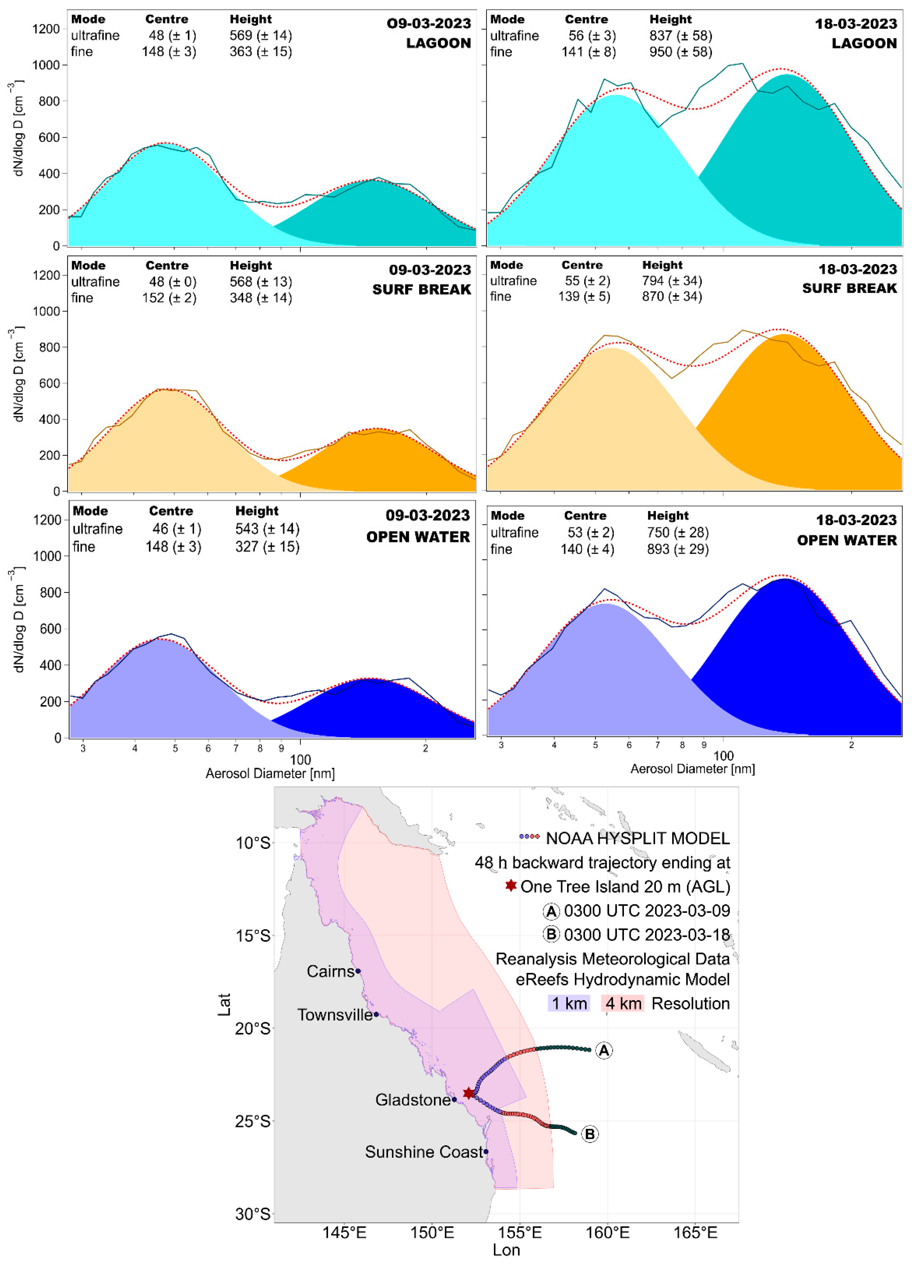
- Stein, A.F.; Draxler, R.R.; Rolph, G.D.; Stunder, B.J.B.; Cohen, M.D.; Ngan, F. NOAA’s HYSPLIT Atmospheric Transport and Dispersion Modeling System. Bull. Am. Meteorol. Soc. 2015, 96, 2059–2077. [Google Scholar] [CrossRef]
- Steven, A.D.; Baird, M.E.; Brinkman, R.; Car, N.J.; Cox, S.J.; Herzfeld, M.; Hodge, J.; Jones, E.; King, E.; Margvelashvili, N. eReefs: An operational information system for managing the Great Barrier Reef. J. Oper. Oceanogr. 2019, 12, S12–S28. [Google Scholar] [CrossRef]
- Schiller, A.; Herzfeld, M.; Brinkman, R.; Rizwi, F.; Andrewartha, J. Cross-shelf exchanges between the Coral Sea and the Great Barrier Reef lagoon determined from a regional-scale numerical model. Cont. Shelf Res. 2015, 109, 150–163. [Google Scholar] [CrossRef]
- Puri, K.; Dietachmayer, G.; Steinle, P.; Dix, M.; Rikus, L.; Logan, L.; Naughton, M.; Tingwell, C.; Xiao, Y.; Barras, V.; et al. Implementation of the initial ACCESS numerical weather prediction system. Aust. Meteorol. Oceanogr. J. 2013, 63, 265–284. [Google Scholar] [CrossRef]
- Kara, A.B.; Wallcraft, A.J.; Metzger, E.J.; Hurlburt, H.E.; Fairall, C.W. Wind Stress Drag Coefficient over the Global Ocean. J. Clim. 2007, 20, 5856–5864. [Google Scholar] [CrossRef]
- Vömel, H. Saturation Vapor Pressure Formulations. Available online: http://cires1.colorado.edu/~voemel/vp.html (accessed on 10 March 2024).
- Huang, X.; Abolt, C.J.; Bennett, K.E. Brief Communication: Effects of different saturation vapor pressure calculations on simulated surface-subsurface hydrothermal regimes at a permafrost field site. Cryosphere Discuss. 2023, 2023, 1–15. [Google Scholar]
- Huang, J. A Simple Accurate Formula for Calculating Saturation Vapor Pressure of Water and Ice. J. Appl. Meteorol. Climatol. 2018, 57, 1265–1272. [Google Scholar] [CrossRef]
- Alduchov, O.A.; Eskridge, R.E. Improved Magnus Form Approximation of Saturation Vapor Pressure. J. Appl. Meteorol. Climatol. 1996, 35, 601–609. [Google Scholar] [CrossRef]
- Textor, C.; Schulz, M.; Guibert, S.; Kinne, S.; Balkanski, Y.; Bauer, S.; Berntsen, T.; Berglen, T.; Boucher, O.; Chin, M.; et al. Analysis and quantification of the diversities of aerosol life cycles within AeroCom. Atmos. Chem. Phys. 2006, 6, 1777–1813. [Google Scholar] [CrossRef]
- Jackson, R.; Gabric, A.; Woodhouse, M.; Swan, H.; Jones, G.; Cropp, R.; Deschaseaux, E. Coral reef emissions of atmospheric dimethylsulfide and the influence on marine aerosols in the southern Great Barrier Reef, Australia. J. Geophys. Res. Atmos. 2020, 125, e2019JD031837. [Google Scholar] [CrossRef]
- Brechtel Manufacturing Inc. Instrument Manual Version 3.4 SEMS 2100. Available online: https://www.brechtel.com/wp-content/uploads/2021/08/bmi_model_2100_SEMS_manual_v3.1.pdf (accessed on 5 February 2024).
- Cochran, R.E.; Laskina, O.; Trueblood, J.V.; Estillore, A.D.; Morris, H.S.; Jayarathne, T.; Sultana, C.M.; Lee, C.; Lin, P.; Laskin, J. Molecular diversity of sea spray aerosol particles: Impact of ocean biology on particle composition and hygroscopicity. Chem 2017, 2, 655–667. [Google Scholar] [CrossRef]
- Ming, Y.; Russell, L.M. Predicted hygroscopic growth of sea salt aerosol. J. Geophys. Res. Atmos. 2001, 106, 28259–28274. [Google Scholar] [CrossRef]
- Choudhury, G.; Ansmann, A.; Tesche, M. Evaluation of aerosol number concentrations from CALIPSO with ATom airborne in situ measurements. Atmos. Chem. Phys. 2022, 22, 7143–7161. [Google Scholar] [CrossRef]
- von der Weiden, S.L.; Drewnick, F.; Borrmann, S. Particle Loss Calculator—A new software tool for the assessment of the performance of aerosol inlet systems. Atmos. Meas. Tech. 2009, 2, 479–494. [Google Scholar] [CrossRef]
- Anderson, M.J. Permutational Multivariate Analysis of Variance (PERMANOVA). In Wiley StatsRef: Statistics Reference Online; Wiley: Hoboken, NJ, USA, 2017; pp. 1–15. [Google Scholar]
- Van Eijk, A.; Kusmierczyk-Michulec, J.; Francius, M.; Tedeschi, G.; Piazzola, J.; Merritt, D.; Fontana, J. Sea-spray aerosol particles generated in the surf zone. J. Geophys. Res. Atmos. 2011, 116, D19210. [Google Scholar] [CrossRef]
- Jackson, R.; Gabric, A.; Matrai, P.; Woodhouse, M.; Cropp, R.; Jones, G.; Deschaseaux, E.; Omori, Y.; McParland, E.; Swan, H. Parameterizing the impact of seawater temperature and irradiance on dimethylsulfide (DMS) in the Great Barrier Reef and the contribution of coral reefs to the global sulfur cycle. J. Geophys. Res. Ocean. 2021, 126, e2020JC016783. [Google Scholar] [CrossRef]
- Hulswar, S.; Simó, R.; Galí, M.; Bell, T.G.; Lana, A.; Inamdar, S.; Halloran, P.R.; Manville, G.; Mahajan, A.S. Third revision of the global surface seawater dimethyl sulfide climatology (DMS-Rev3). Earth Syst. Sci. Data 2022, 14, 2963–2987. [Google Scholar] [CrossRef]
- Lana, A.; Bell, T.G.; Simó, R.; Vallina, S.M.; Ballabrera-Poy, J.; Kettle, A.J.; Dachs, J.; Bopp, L.; Saltzman, E.S.; Stefels, J.; et al. An updated climatology of surface dimethlysulfide concentrations and emission fluxes in the global ocean. Glob. Biogeochem. Cycles 2011, 25, GB1004. [Google Scholar] [CrossRef]
- Saliba, G.; Chen, C.-L.; Lewis, S.; Russell, L.M.; Rivellini, L.-H.; Lee, A.K.Y.; Quinn, P.K.; Bates, T.S.; Haëntjens, N.; Boss, E.S.; et al. Factors driving the seasonal and hourly variability of sea-spray aerosol number in the North Atlantic. Proc. Natl. Acad. Sci. USA 2019, 116, 20309–20314. [Google Scholar] [CrossRef]
- Zinke, J.; Nilsson, E.D.; Zieger, P.; Salter, M.E. The effect of seawater salinity and seawater temperature on sea salt aerosol production. J. Geophys. Res. Atmos. 2022, 127, e2021JD036005. [Google Scholar] [CrossRef]
- Land, P.E.; Shutler, J.D.; Bell, T.; Yang, M. Exploiting satellite earth observation to quantify current global oceanic DMS flux and its future climate sensitivity. J. Geophys. Res. Ocean. 2014, 119, 7725–7740. [Google Scholar] [CrossRef]
- Lv, C.; Tsona, N.T.; Du, L. Sea spray aerosol formation: Results on the role of different parameters and organic concentrations from bubble bursting experiments. Chemosphere 2020, 252, 126456. [Google Scholar] [CrossRef] [PubMed]
- Girdwood, J.; Smith, H.; Stanley, W.; Ulanowski, Z.; Stopford, C.; Chemel, C.; Doulgeris, K.M.; Brus, D.; Campbell, D.; Mackenzie, R. Design and field campaign validation of a multi-rotor unmanned aerial vehicle and optical particle counter. Atmos. Meas. Tech. 2020, 13, 6613–6630. [Google Scholar] [CrossRef]
- Bilyeu, L.; Bloomfield, B.; Hanlon, R.; González-Rocha, J.; Jacquemin, S.J.; Ault, A.P.; Birbeck, J.A.; Westrick, J.A.; Foroutan, H.; Ross, S.D. Drone-based particle monitoring above two harmful algal blooms (HABs) in the USA. Environ. Sci. Atmos. 2022, 2, 1351–1363. [Google Scholar] [CrossRef]
- Bieber, P.; Seifried, T.M.; Burkart, J.; Gratzl, J.; Kasper-Giebl, A.; Schmale, D.G.; Grothe, H. A Drone-Based Bioaerosol Sampling System to Monitor Ice Nucleation Particles in the Lower Atmosphere. Remote Sens. 2020, 12, 552. [Google Scholar] [CrossRef]
- Bretschneider, L.; Schlerf, A.; Baum, A.; Bohlius, H.; Buchholz, M.; Düsing, S.; Ebert, V.; Erraji, H.; Frost, P.; Käthner, R.; et al. MesSBAR—Multicopter and Instrumentation for Air Quality Research. Atmosphere 2022, 13, 629. [Google Scholar] [CrossRef]
- Liu, Z.; Osborne, M.; Anderson, K.; Shutler, J.D.; Wilson, A.; Langridge, J.; Yim, S.H.L.; Coe, H.; Babu, S.; Satheesh, S.K.; et al. Characterizing the performance of a POPS miniaturized optical particle counter when operated on a quadcopter drone. Atmos. Meas. Tech. 2021, 14, 6101–6118. [Google Scholar] [CrossRef]
- Brechtel Manufacturing Inc. Instrument Manual Ver. 2.0 mini-OPC 9405 For UAV Reader Version 8.1 and Firmware Version 3.1; Brechtel Manufacturing Inc.: Hayward, CA, USA, 2023. [Google Scholar]
- Karagulian, F.; Barbiere, M.; Kotsev, A.; Spinelle, L.; Gerboles, M.; Lagler, F.; Redon, N.; Crunaire, S.; Borowiak, A. Review of the performance of low-cost sensors for air quality monitoring. Atmosphere 2019, 10, 506. [Google Scholar] [CrossRef]
- Snider, J.R.; Petters, M.D. Optical particle counter measurement of marine aerosol hygroscopic growth. Atmos. Chem. Phys. 2008, 8, 1949–1962. [Google Scholar] [CrossRef]
- Wang, Y.-C.; Wang, S.-H.; Lewis, J.R.; Chang, S.-C.; Griffith, S.M. Determining planetary boundary layer height by micro-pulse lidar with validation by UAV measurements. Aerosol Air Qual. Res. 2021, 21, 200336. [Google Scholar] [CrossRef]


| MIN | MAX | MEAN | ±SD | |
|---|---|---|---|---|
| Total wind stress magnitude [Pa] | 0.003 | 0.158 | 0.050 | 0.037 |
| Air–water temperature [°C] | −3.1 | 1.2 | −1.0 | 0.9 |
| Salinity | 34.95 | 35.60 | 35.20 | 0.13 |
| Mixing depth [m] | 250 | 936 | 446 | 212 |
| Relative humidity [%] | 70 | 94 | 83 | 5 |
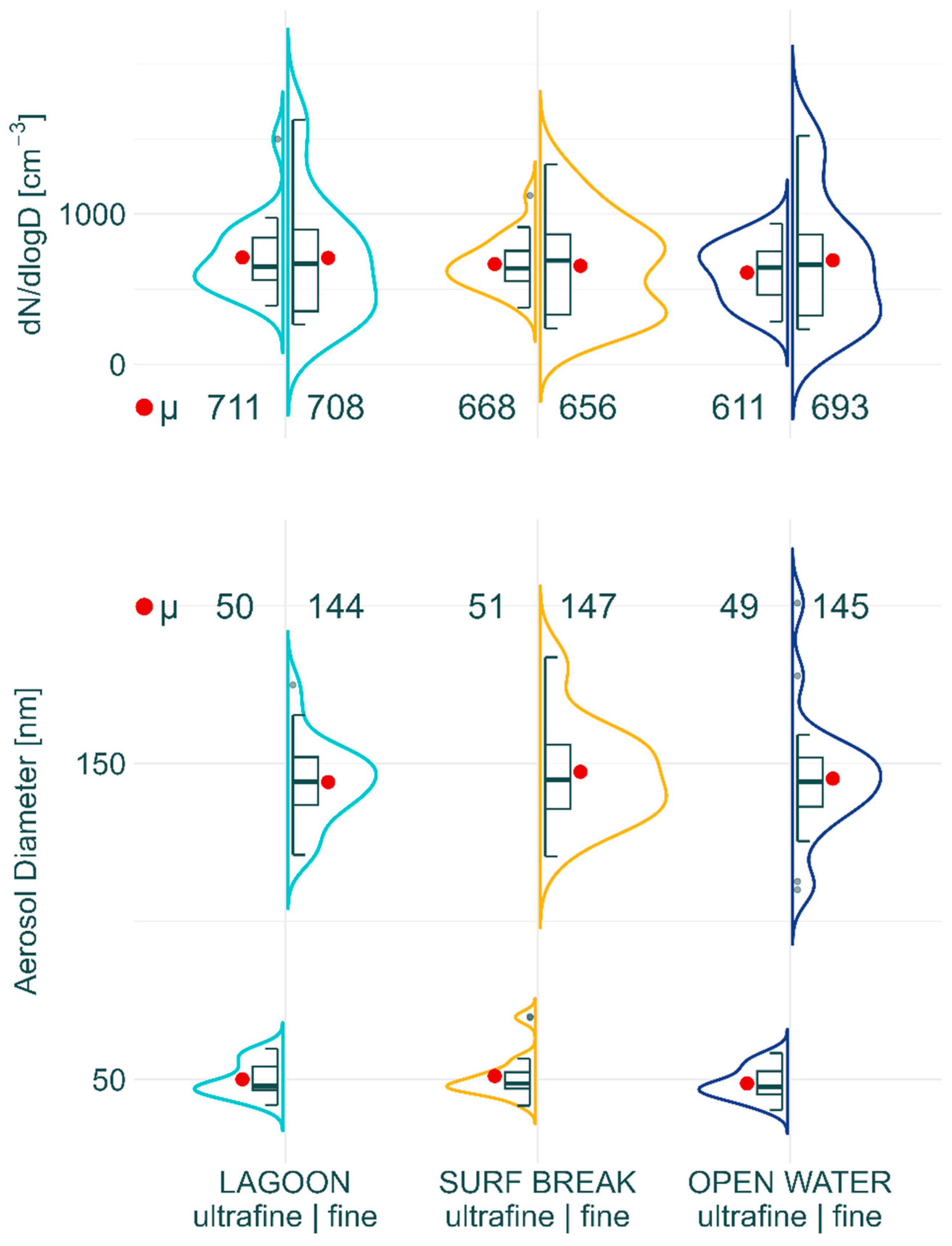
| Height [dN/dlogD [cm⁻3]] | ultrafine|fine | |||
| Lagoon | 392|267 | 1498|1625 | 711|708 | 251|408 |
| Surf break | 377|240 | 1123|1329 | 668|656 | 175|328 |
| Open water | 284|235 | 935|1519 | 611|693 | 196|422 |
| Centre [nm] | ||||
| Lagoon | 42|121 | 60|175 | 50|144 | 5|13 |
| Surf break | 42|121 | 70|184 | 51|147 | 7|16 |
| Open water | 40|110 | 58|201 | 49|145 | 5|20 |
| PERMANOVA (Ultrafine|Fine) | |||
|---|---|---|---|
| df | Pseudo-F | p | |
| Location (Fixed) | 2|2 | 3.237|1.832 | 0.037|0.183 |
| Day (Random) | 9|9 | 12.373|115.57 | 0.0001|0.0001 |
| PAIRWISE TESTS (ultrafine) | |||
| Pseudo-t | p | ||
| Lagoon–Surf break | 0.974 | 0.3546 | |
| Lagoon–Open water | 2.444 | 0.0146 | |
| Surf Break–Open water | 2.088 | 0.0423 | |
| DISTANCE BASED LINEAR MODEL (ultrafine|fine) | |||
| MARGINAL TESTS | R2 | p | |
| Total wind stress magnitude | 0.03|0.00 | 0.1955|0.8012 | |
| Air–water temperature | 0.34|0.40 | 0.0001|0.0001 | |
| Salinity | 0.12|0.14 | 0.0056|0.0044 | |
| BEST SOLUTIONS (ultrafine) | R2 | AICc | |
| Air–water temperature | 0.34 | 620.14 | |
| Air–water temperature, salinity | 0.34 | 622.24 | |
| BEST SOLUTIONS (fine) | |||
| Air–water temperature | 0.40 | 685.92 | |
| Total wind stress magnitude, air–water temperature | 0.42 | 686.48 | |
Disclaimer/Publisher’s Note: The statements, opinions and data contained in all publications are solely those of the individual author(s) and contributor(s) and not of MDPI and/or the editor(s). MDPI and/or the editor(s) disclaim responsibility for any injury to people or property resulting from any ideas, methods, instructions or products referred to in the content. |
© 2024 by the authors. Licensee MDPI, Basel, Switzerland. This article is an open access article distributed under the terms and conditions of the Creative Commons Attribution (CC BY) license (https://creativecommons.org/licenses/by/4.0/).
Share and Cite
Eckert, C.; Hernandez-Jaramillo, D.C.; Medcraft, C.; Harrison, D.P.; Kelaher, B.P. Drone-Based Measurement of the Size Distribution and Concentration of Marine Aerosols above the Great Barrier Reef. Drones 2024, 8, 292. https://doi.org/10.3390/drones8070292
Eckert C, Hernandez-Jaramillo DC, Medcraft C, Harrison DP, Kelaher BP. Drone-Based Measurement of the Size Distribution and Concentration of Marine Aerosols above the Great Barrier Reef. Drones. 2024; 8(7):292. https://doi.org/10.3390/drones8070292
Chicago/Turabian StyleEckert, Christian, Diana C. Hernandez-Jaramillo, Chris Medcraft, Daniel P. Harrison, and Brendan P. Kelaher. 2024. "Drone-Based Measurement of the Size Distribution and Concentration of Marine Aerosols above the Great Barrier Reef" Drones 8, no. 7: 292. https://doi.org/10.3390/drones8070292