maths revision to help you

Copyright © 2006 AQA and its licensors. All rights reserved.
Version 1.0 0306 klm
GCE Mathematics (6360)
Further Pure unit 4 (MFP4)
Textbook
The Assessment and Qualifications Alliance (AQA) is a company limited by guarantee registered in England and Wales 3644723 and a registered charity number 1073334.
Registered address AQA, Devas Street, Manchester M15 6EX. Dr Michael Cresswell Director General.

klmGCE Mathematics (6360) Further Pure 4 (MFP4) Textbook
2
Further Pure 4: Contents
Chapter 1: Matrix algebra 3
1.1 Matrices 4
1.2 Matrix arithmetic 5
1.3 Laws of matrix arithmetic 10
1.4 Matrix transformations (2-dimensional) 13
1.5 Linear transformations 15
1.6 Matrix transformations (2-dimensional) 20
Chapter 2: The vector product 25
2.1 Introduction 26
2.2 Properties of the vector product 27
2.3 Vector products in component form 28
2.4 Application of vector products to areas 30
2.5 Triple products 31
2.6 Properties of scalar triple products 32
2.7 Proof of the distributive law 33
Chapter 3: Determinants 35
3.1 Directed areas 36
3.2 2 2× determinants 37
3.3 3 3× determinants 39
3.4 A general formula 40
3.5 Rules for manipulating determinants 42
3.6 Determinants of products 45
Chapter 4: Applications of vector products 47
4.1 Calculation of vector products in practice 48
4.2 Volumes 49
4.3 Coplanarity of vectors 52
4.4 Equations of lines 54
4.5 Equations of planes 58
4.6 Angles between lines and planes 63
4.7 Shortest distances 65
Chapter 5: Inverse matrices 72
5.1 Inverses 73
5.2 2 2× matrices 74
5.3 3 3× matrices 75
5.4 Products 78
Chapter 6: Solving linear equations 81
6.1 Geometrical interpretation 82
6.2 Inverse matrices 84
6.3 Row operations 86
6.4 Linear independence 88
Chapter 7: Eigenvectors 96
7.1 Invariant points and lines 97
7.2 Eigenvectors and eigenvalues 100
7.3 The characteristic equation 101
7.4 Diagonalisation 105
Answers to the exercises in Further Pure 3 114

3
Chapter 1: Matrix Algebra
1.1 Matrices
1.2 Matrix arithmetic
1.3 Laws of matrix arithmetic
1.4 Matrix transformations (2-dimensional)
1.5 Linear transformations
This chapter introduces the idea of a matrix. When you have completed it, you will:
• know what is meant by a matrix;
• be able to add, subtract and multiply matrices;
• be able to multiply matrices by scalars;
• know what is meant by the transpose of a matrix;
• understand how matrices can represent transformations;
• know the matrices for some transformations;
• be able to calculate the matrices for combined transformations.

4
1.1 Matrices
Any rectangular array of numbers is called a matrix (the plural is matrices).
For example,
1 3
3 5
4 1
−⎡ ⎤
⎢ ⎥= ⎢ ⎥
⎢ ⎥−⎣ ⎦
M
is a matrix. M has three rows and two columns and is called a matrix of order ×3 2 or,
simply, a ×3 2 matrix. Note that each row or column is itself a matrix. For example, the
third row is [ ]4 1− , a 1 2× matrix.
Each number in a matrix is called an element.
Exercise 1A
In the following questions, A is the matrix defined by
3 1 2 1
.
1 1 1 4
−⎡ ⎤
= ⎢ ⎥−⎣ ⎦
A
1. What is the order of matrix A?
2. Which element of A is in the first row and in the third column?
3. What type of matrix is the fourth column of A?
4. A triangle has coordinates (3, 4), (–1, 2), (2, –3). Represent this triangle by a 2 3× matrix
with the coordinates forming the columns.
When giving the order of a matrix, you should always give
the number of rows first, then the number of columns

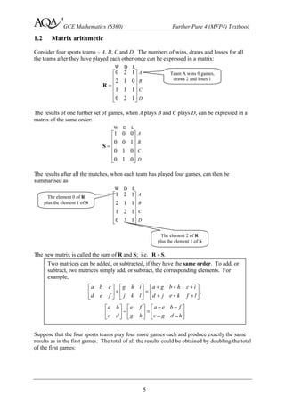
5
1.2 Matrix arithmetic
Consider four sports teams – A, B, C and D. The numbers of wins, draws and losses for all
the teams after they have played each other once can be expressed in a matrix:
0 2 1
2 1 0
1 1 1
0 2 1
⎡ ⎤
⎢ ⎥
⎢ ⎥=
⎢ ⎥
⎢ ⎥
⎣ ⎦
R
The results of one further set of games, when A plays B and C plays D, can be expressed in a
matrix of the same order:
1 0 0
0 0 1
0 1 0
0 1 0
⎡ ⎤
⎢ ⎥
⎢ ⎥=
⎢ ⎥
⎢ ⎥
⎣ ⎦
S
The results after all the matches, when each team has played four games, can then be
summarised as
1 2 1
2 1 1
1 2 1
0 3 1
⎡ ⎤
⎢ ⎥
⎢ ⎥
⎢ ⎥
⎢ ⎥
⎣ ⎦
The new matrix is called the sum of R and S; i.e. .+R S
Suppose that the four sports teams play four more games each and produce exactly the same
results as in the first games. The total of all the results could be obtained by doubling the total
of the first games:
W D L
A
B
C
D
W D L
A
B
C
D
W D L
A
B
C
D
The element 0 of R
plus the element 1 of S
The element 2 of R
plus the element 1 of S
Two matrices can be added, or subtracted, if they have the same order. To add, or
subtract, two matrices simply add, or subtract, the corresponding elements. For
example,
,
a b c g h i a g b h c i
d e f j k l d j e k f l
+ + +⎡ ⎤ ⎡ ⎤ ⎡ ⎤
+ =⎢ ⎥ ⎢ ⎥ ⎢ ⎥+ + +⎣ ⎦ ⎣ ⎦ ⎣ ⎦
a b e f a e b f
c d g h c g d h
− −⎡ ⎤ ⎡ ⎤ ⎡ ⎤
− =⎢ ⎥ ⎢ ⎥ ⎢ ⎥− −⎣ ⎦ ⎣ ⎦ ⎣ ⎦
Team A wins 0 games,
draws 2 and loses 1

6
1 2 1 2 4 2
2 1 1 4 2 2
2 .
1 2 1 2 4 2
0 3 1 0 6 2
⎡ ⎤ ⎡ ⎤
⎢ ⎥ ⎢ ⎥
⎢ ⎥ ⎢ ⎥=
⎢ ⎥ ⎢ ⎥
⎢ ⎥ ⎢ ⎥
⎣ ⎦ ⎣ ⎦
When calculating with matrices, ordinary numbers are called scalars. Multiplication of a
matrix by a scalar, as above, is called scalar multiplication.
Suppose that the method of awarding points to teams is 3 for a win, 1 for a draw and 0 for a
loss. The points can be expressed in a 3 1× matrix,
3
1
0
⎡ ⎤
⎢ ⎥
⎢ ⎥
⎢ ⎥⎣ ⎦
The total number of points earned by each team, when each has played eight games, can be
found as follows.
Results Points
2 4 2
4 2 2
2 4 2
0 6 2
⎡ ⎤
⎢ ⎥
⎢ ⎥
⎢ ⎥
⎢ ⎥
⎣ ⎦
3
1
0
⎡ ⎤
⎢ ⎥
⎢ ⎥
⎢ ⎥⎣ ⎦
10
14
10
6
⎡ ⎤
⎢ ⎥
⎢ ⎥
⎢ ⎥
⎢ ⎥
⎣ ⎦
Now suppose that there are two methods of awarding points to teams.
! Method I : 3 points for a win; 1 point for a draw; 0 for a loss.
! Method II : 2 points for a win; 1 point for a draw; 0 for a loss.
These two possibilities can also be expressed as a matrix:
3 2
1 1
0 0
⎡ ⎤
⎢ ⎥
⎢ ⎥
⎢ ⎥⎣ ⎦
Any matrix can be multiplied by any scalar. Simply multiply
each element by the scalar. For example,
a b ka kb
k c d kc kd
e f ke kf
⎡ ⎤ ⎡ ⎤
⎢ ⎥ ⎢ ⎥=⎢ ⎥ ⎢ ⎥
⎢ ⎥ ⎢ ⎥⎣ ⎦ ⎣ ⎦
I II
W
D
L
W
D
L
A
B
C
D
W
D
L
Team A earned
(2 3) (4 1) (2 0) 10× + × + × = points
A
B
C
D

7
The two possibilities for the total number of points earned by each team after each team has
played eight games are found as follows.
2 4 2
4 2 2
2 4 2
0 6 2
⎡ ⎤
⎢ ⎥
⎢ ⎥
⎢ ⎥
⎢ ⎥
⎣ ⎦
3 2
1 1
0 0
⎡ ⎤
⎢ ⎥
⎢ ⎥
⎢ ⎥⎣ ⎦
10 8
14 10
10 8
6 6
⎡ ⎤
⎢ ⎥
⎢ ⎥
⎢ ⎥
⎢ ⎥
⎣ ⎦
This combination of the 4 3× matrix of results and the 3 2× matrix of points is called matrix
multiplication, i.e.
2 4 2 10 8
3 2
4 2 2 14 10
1 1 .
2 4 2 10 8
0 0
0 6 2 6 6
⎡ ⎤ ⎡ ⎤
⎡ ⎤⎢ ⎥ ⎢ ⎥
⎢ ⎥⎢ ⎥ ⎢ ⎥× =⎢ ⎥⎢ ⎥ ⎢ ⎥
⎢ ⎥⎢ ⎥ ⎢ ⎥⎣ ⎦
⎣ ⎦ ⎣ ⎦
To multiply two matrices, the number of columns in the first matrix must equal the number of
rows in the second matrix. This is because of the way that pairs of numbers are multiplied.
For example, the second row of the 4 3× matrix above is multiplied by the first column of the
3 2× matrix as follows:
W
D
L
W D L
A
B
C
D
I II
I II
A
B
C
D
(2 3) (4 1) (2 0)× + × + ×
(4 2) (2 1) (2 0)× + × + ×
4 2 2
0
1
3
14)02()12()34( =×+×+×

8
Consider the orders of the matrices in the example above.
left hand matrix × right hand matrix product matrix
4 3× 3 2× 4 2×
Example 1.2.1
If
2 1
1 3
⎡ ⎤
= ⎢ ⎥−⎣ ⎦
A and
1 1
2 3 ,
1 2
−⎡ ⎤
⎢ ⎥= ⎢ ⎥
⎢ ⎥⎣ ⎦
B find which of the products AB and BA can be evaluated.
Solution
A is 2 2× and B is 3 2.× Hence,
2 2× 3 2× so AB cannot be evaluated;
3 2× 2 2× so BA can be evaluated and is 3 2.×
1 1 1 4
2 1
2 3 7 7
1 3
1 2 4 5
−⎡ ⎤ ⎡ ⎤
⎡ ⎤⎢ ⎥ ⎢ ⎥= = −⎢ ⎥⎢ ⎥ ⎢ ⎥−⎣ ⎦⎢ ⎥ ⎢ ⎥−⎣ ⎦ ⎣ ⎦
BA
these numbers must be equal
these numbers determine the
order of the product matrix
Matrices are multiplied by multiplying the elements in a row of the first matrix by
the elements in a column of the second matrix, and adding the results. For
example,
a b ag bk ah bl ai bm aj bn
g h i j
c d cg dk ch dl ci dm cj dn
k l m n
e f eg fk eh fl ei fm ej fn
+ + + +⎡ ⎤ ⎡ ⎤
⎡ ⎤⎢ ⎥ ⎢ ⎥= + + + +⎢ ⎥⎢ ⎥ ⎢ ⎥
⎣ ⎦⎢ ⎥ ⎢ ⎥+ + + +⎣ ⎦ ⎣ ⎦
The product AB can be found if the number of columns of matrix A is equal to the
number of rows of matrix B. If the order of matrix A is r s× and B is s t× , then
the order of AB is r t×
different
equal
(1 1) ( 1 3)× + − × −

9
Exercise 1B
1. If
3 1 1
1 2 0
−⎡ ⎤
= ⎢ ⎥
⎣ ⎦
A and
1 1
1 0 ,
2 1
−⎡ ⎤
⎢ ⎥= ⎢ ⎥
⎢ ⎥⎣ ⎦
B find AB and BA.
2.
1 2
2 1
−⎡ ⎤
= ⎢ ⎥
⎣ ⎦
A and
2 2
.
1 3
⎡ ⎤
= ⎢ ⎥−⎣ ⎦
B
(a) Find 2 2
, , and .A B AB BA
(b) Find +A B and verify that 2 2 2
( ) .+ = + + +A B A AB BA B
3. Which of the following matrices can be multiplied by themselves?
[ ]
1 1 3 1 1
1 0
3 1 , 1 1 2 , 1 1 4 , .
0 1
1 2 2 1 3
−⎡ ⎤ ⎡ ⎤
⎡ ⎤⎢ ⎥ ⎢ ⎥= = − = = ⎢ ⎥⎢ ⎥ ⎢ ⎥
⎣ ⎦⎢ ⎥ ⎢ ⎥−⎣ ⎦ ⎣ ⎦
A B C D
4. Let
2 1
3 1
⎡ ⎤
= ⎢ ⎥−⎣ ⎦
A and
1 0
.
0 1
⎡ ⎤
= ⎢ ⎥
⎣ ⎦
I Show that 2
5 .= +A A I
5. Let [ ]
1 1
1 2
1 1 2 , 2 1 and .
2 1
1 3
−⎡ ⎤
⎡ ⎤⎢ ⎥= − = = ⎢ ⎥⎢ ⎥ −⎣ ⎦⎢ ⎥⎣ ⎦
A B C Show that ( ) ( ).=AB C A BC
6. A is a 1 3× matrix and B is a 4 2× matrix. Given that the products AX, XB, BY and YA
can all be found, what are the orders of X and Y?
7. Given that
2 1 1 1 2 2 0 1
, and ,
1 1 3 0 1 1 1 3
−⎡ ⎤ ⎡ ⎤ ⎡ ⎤
= = =⎢ ⎥ ⎢ ⎥ ⎢ ⎥− −⎣ ⎦ ⎣ ⎦ ⎣ ⎦
A B C find ( ),+A B C
AB and AC.
What do you notice?
8. Find
2 1 1 2 0 1
1 3 2 1 3 1 .
3 1 2 2 1 0
− −⎡ ⎤ ⎡ ⎤
⎢ ⎥ ⎢ ⎥−⎢ ⎥ ⎢ ⎥
⎢ ⎥ ⎢ ⎥− −⎣ ⎦ ⎣ ⎦

10
1.3 Laws of matrix arithmetic
Since the addition of two matrices simply involves the addition of corresponding elements,
matrix addition is itself straightforward. In particular:
As you have seen in Exercise 1B, matrix multiplication is not so straightforward.
However, in two important respects, matrix arithmetic and ordinary arithmetic are very
similar. Firstly, you can expand brackets in the usual way.
Secondly, in a string of matrix multiplications, although you must not change the sequence of
the matrices, you can multiply any adjacent pair together first. Consequently, you can write a
product such as ABC without ambiguity.
A zero matrix is any matrix consisting entirely of zeros. Any such matrix is denoted by 0.
For example, [ ]0 0 .=0
Commutativity of addition
For any two matrices which can be added (i.e. which
have the same order), + = +A B B A
Non-commutativity of multiplication
It cannot be assumed that ,=AB BA even when both products exist
Distributive law
For any matrices of appropriate orders,
( ) ,
( )
+ = +
+ = +
A B C AB AC
U V W UW VW
Associative law
For any matrices of appropriate orders,
( ) ( )=A BC AB C
For all matrices of suitable orders,
, and+ = = =A 0 A 0B 0 C0 0

11
An identity matrix is any square matrix in which all of the elements on the leading diagonal
are 1 and all other elements are zeros. Such a matrix is denoted by I. For example,
1 0 0 0
1 0 0 1 0 0
or .
0 1 0 0 1 0
0 0 0 1
⎡ ⎤
⎢ ⎥
⎡ ⎤ ⎢ ⎥= =⎢ ⎥ ⎢ ⎥⎣ ⎦
⎢ ⎥
⎣ ⎦
I I
In particular, for any square matrix M of the same order as I, .= =MI IM M
In some circumstances it can be useful to interchange the rows and columns of a matrix. This
process is called transposing the matrix.
Example 1.3.1
Given that
1 2 1 2 1
2 1 1 and 1 4 ,
3 4 2 0 2
−⎡ ⎤ ⎡ ⎤
⎢ ⎥ ⎢ ⎥= − = −⎢ ⎥ ⎢ ⎥
⎢ ⎥ ⎢ ⎥−⎣ ⎦ ⎣ ⎦
A B
find (a) AB, (b) AT
, (c) BT
and (d) BT
AT
.
(e) What do you notice about AB and BT
AT
?
Solution
0 9
5 4 .
2 9
⎡ ⎤
⎢ ⎥= −⎢ ⎥
⎢ ⎥⎣ ⎦
AB T
1 2 3
2 1 4 .
1 1 2
⎡ ⎤
⎢ ⎥= −⎢ ⎥
⎢ ⎥−⎣ ⎦
A
T 2 01
.
1 4 2
−⎡ ⎤
= ⎢ ⎥−⎣ ⎦
B T T 0 5 2
.
9 4 9
⎡ ⎤
= ⎢ ⎥−⎣ ⎦
B A
BT
AT
is the same as (AB)T
.
The result noted in part (e) of Example 1.3.1 is true for all compatible matrices A and B.
For all matrices of suitable orders,
and= =AI A IB B
The transpose of a matrix M is obtained by interchanging the
rows and columns of M. The transpose of M is denoted by MT
T T T
( ) =AB B A
(a) (b)
(c) (d)
(e)

12
Exercise 1C
1. Given that A is the matrix
2 1
,
6 3
−⎡ ⎤
⎢ ⎥−⎣ ⎦
find a non-zero matrix B such that .=AB 0
2. Find two non-zero matrices, A and B, such that .= =AB BA 0
3. Let
1 2 4 8
and .
1 3 1 6
⎡ ⎤ ⎡ ⎤
= =⎢ ⎥ ⎢ ⎥− −⎣ ⎦ ⎣ ⎦
A B Solve for X the equation 3 .+ =A X B
4. Let
1 0
.
0 0
⎡ ⎤
= ⎢ ⎥
⎣ ⎦
A Find all matrices B such that .=AB BA
5. The matrices A, B, C, M and N are such that
and .= =M AB N BC
Explain why .=AN MC
6. The matrices A, B and C are such that
3 1 5 1
and .
2 8 7 5
⎡ ⎤ ⎡ ⎤
= =⎢ ⎥ ⎢ ⎥
⎣ ⎦ ⎣ ⎦
AB AC
Find ( ).−A B C
7. Check the result T T T
( ) =AB B A for the matrices
2 1
3 1 2
, 5 1 .
2 0 1
0 3
−⎡ ⎤
−⎡ ⎤ ⎢ ⎥= = −⎢ ⎥ ⎢ ⎥
⎣ ⎦ ⎢ ⎥⎣ ⎦
A B

13
An important area of application of matrices is that of geometrical transformations. Consider
the matrix multiplication of any 2 2× matrix by a 2 1× matrix – for example,
0 1 3 4
1 0 4 3
− −⎡ ⎤ ⎡ ⎤ ⎡ ⎤
=⎢ ⎥ ⎢ ⎥ ⎢ ⎥
⎣ ⎦ ⎣ ⎦ ⎣ ⎦
You can think of the 2 1× matrices as representing the points (3, 4) and (–4, 3), respectively.
The 2 2× matrix then represents a transformation which maps P(3, 4) onto P′ (–4, 3).
Example 1.4.1
(a) A rectangle has vertices O(0, 0), A(3, 0), B(3, 1) and C(0, 1). Find the images O′, A′, B′
and C′ of these points when acted on by the transformation represented by the matrix
0 1
.
1 0
−⎡ ⎤
= ⎢ ⎥
⎣ ⎦
M
(b) Hence describe the transformation represented by M.
Solution
0 1 0 3 3 0 0 0 1 1
1 0 0 0 1 1 0 3 3 0
− − −⎡ ⎤ ⎡ ⎤ ⎡ ⎤
=⎢ ⎥ ⎢ ⎥ ⎢ ⎥
⎣ ⎦ ⎣ ⎦ ⎣ ⎦
M represents a rotation of 90°
anticlockwise about the origin O.
Write each point as a
column of a single matrix
(–1, 3) is the image of (3, 1)
Any 2 2× matrix M can be thought of as representing a
geometrical transformation of the points in the plane.
To find the image of any point (a, b), find
a
b
⎡ ⎤
⎢ ⎥
⎣ ⎦
M
B′
A′
C B
C′ AO=O′
(a)
(b)

14
This table lists some simple matrices and the geometrical transformations they represent.
1 0
0 1
⎡ ⎤
⎢ ⎥
⎣ ⎦
Identity: all points unchanged
0 1
1 0
−⎡ ⎤
⎢ ⎥
⎣ ⎦
Rotation of 90° anticlockwise about O
1 0
0 1
−⎡ ⎤
⎢ ⎥−⎣ ⎦
Rotation of 180° about O
0 1
1 0
⎡ ⎤
⎢ ⎥−⎣ ⎦
Rotation of 90° clockwise about O
1 0
0 1
⎡ ⎤
⎢ ⎥−⎣ ⎦
Reflection in the x-axis
1 0
0 1
−⎡ ⎤
⎢ ⎥
⎣ ⎦
Reflection in the y-axis
0 1
1 0
⎡ ⎤
⎢ ⎥
⎣ ⎦
Reflection in the line y x=
2 0
0 2
⎡ ⎤
⎢ ⎥
⎣ ⎦
An enlargement, 2,× centre at O
3 0
0 1
⎡ ⎤
⎢ ⎥
⎣ ⎦
A stretch, 3,× from the y-axis
1 0
0 4
⎡ ⎤
⎢ ⎥
⎣ ⎦
A stretch, 4,× from the x-axis
1 1
0 1
⎡ ⎤
⎢ ⎥
⎣ ⎦
A shear, parallel to the x-axis
Transformations represented by matrices can be combined by multiplying the matrices in a
special order. Suppose you want to transform a point
x
y
⎡ ⎤
⎢ ⎥
⎣ ⎦
first by the transformation
represented by A, and then by the transformation represented by B.
x
y
⎡ ⎤
⎢ ⎥
⎣ ⎦
would become
x
y
⎡ ⎤
⎢ ⎥
⎣ ⎦
A and then .
x
y
⎛ ⎞⎡ ⎤
⎜ ⎟⎢ ⎥
⎣ ⎦⎝ ⎠
B A By the associativity of matrix multiplication,
( ) .
x x
y y
⎛ ⎞⎡ ⎤ ⎡ ⎤
=⎜ ⎟⎢ ⎥ ⎢ ⎥
⎣ ⎦ ⎣ ⎦⎝ ⎠
B A BA
The matrix BA represents the transformation A followed by the transformation B

15
Example 1.4.2
Find the matrix which represents a rotation of 90° anticlockwise about O, followed by a
reflection in the x-axis, followed by a shear parallel to the x-axis such that (0, 1) is
transformed to (1, 1).
Solution
Successively multiply any point (a, b) by the matrices
0 1
,
1 0
−⎡ ⎤
⎢ ⎥
⎣ ⎦
1 0
0 1
⎡ ⎤
⎢ ⎥−⎣ ⎦
and
1 1
.
0 1
⎡ ⎤
⎢ ⎥
⎣ ⎦
By associativity,
1 1 1 0 0 1 1 1 1 0 0 1
.
0 1 0 1 1 0 0 1 0 1 1 0
a a
b b
⎧ ⎫⎛ ⎞ ⎛ ⎞− −⎡ ⎤ ⎡ ⎤ ⎡ ⎤ ⎡ ⎤ ⎡ ⎤ ⎡ ⎤ ⎡ ⎤ ⎡ ⎤⎪ ⎪
=⎨ ⎜ ⎟⎬ ⎜ ⎟⎢ ⎥ ⎢ ⎥ ⎢ ⎥ ⎢ ⎥ ⎢ ⎥ ⎢ ⎥ ⎢ ⎥ ⎢ ⎥− −⎣ ⎦ ⎣ ⎦ ⎣ ⎦ ⎣ ⎦ ⎣ ⎦ ⎣ ⎦ ⎣ ⎦ ⎣ ⎦⎪ ⎪⎝ ⎠ ⎝ ⎠⎩ ⎭
The single matrix is therefore
1 1 0 1 1 1
.
0 1 1 0 1 0
− − −⎡ ⎤ ⎡ ⎤ ⎡ ⎤
=⎢ ⎥ ⎢ ⎥ ⎢ ⎥− −⎣ ⎦ ⎣ ⎦ ⎣ ⎦
1.5 Linear transformations
A matrix such as
2 1
1 1
⎡ ⎤
= ⎢ ⎥−⎣ ⎦
M maps the unit vectors as shown:
2 1 1 2
: 2 ,
1 1 0 1
2 1 0 1
: .
1 1 1 1
⎡ ⎤ ⎡ ⎤ ⎡ ⎤
→ = = −⎢ ⎥ ⎢ ⎥ ⎢ ⎥− −⎣ ⎦ ⎣ ⎦ ⎣ ⎦
⎡ ⎤ ⎡ ⎤ ⎡ ⎤
→ = = +⎢ ⎥ ⎢ ⎥ ⎢ ⎥−⎣ ⎦ ⎣ ⎦ ⎣ ⎦
M i i j
M j i j
Any point, say P, on the usual Cartesian grid is then mapped onto the corresponding point, P′,
on a grid of parallelograms defined by 2 and .− +i j i j
O
y
x
P
O
y
x
P′

16
Any transformation which maps the Cartesian grid of straight lines onto another such grid of
parallel straight lines is called a linear transformation. A more formal definition is given
below.
Typical linear transformations are rotations about the origin, reflections in lines through the
origin, stretches and shears.
Any linear transformation can be represented by a square matrix. Furthermore, as illustrated
by the matrix M at the start of this section,
Example 1.5.1
Find the matrix M representing a shear parallel to the y-axis such that (1, 0) (1, 4).→
Solution
1 1 0 0 1 0
and , so .
0 4 1 1 4 1
⎡ ⎤ ⎡ ⎤ ⎡ ⎤ ⎡ ⎤ ⎡ ⎤
→ → =⎢ ⎥ ⎢ ⎥ ⎢ ⎥ ⎢ ⎥ ⎢ ⎥
⎣ ⎦ ⎣ ⎦ ⎣ ⎦ ⎣ ⎦ ⎣ ⎦
M
A linear transformation has the following properties:
For any vectors a and b, and any scalar λ,
T( ) T( ),
T( ) T( ) T( )
λ λ=
+ = +
a a
a b a b
The matrix representing a given linear transformation in two dimensions
is ,
a b
c d
⎡ ⎤
⎢ ⎥
⎣ ⎦
where the first column is the image of i and the second
column is the image of j

17
Example 1.5.2
Find the matrix R which represents an anticlockwise rotation of θ about the origin.
Solution
1 cos 0 sin
and .
0 sin 1 cos
θ θ
θ θ
−⎡ ⎤ ⎡ ⎤ ⎡ ⎤ ⎡ ⎤
→ →⎢ ⎥ ⎢ ⎥ ⎢ ⎥ ⎢ ⎥
⎣ ⎦ ⎣ ⎦ ⎣ ⎦ ⎣ ⎦
So,
cos sin
.
sin cos
θ θ
θ θ
−⎡ ⎤
= ⎢ ⎥
⎣ ⎦
R
Example 1.5.3
Find the matrix M which represents a reflection in the line tan .y θ=
Solution
1 cos2
0 sin 2
θ
θ
⎡ ⎤ ⎡ ⎤
→⎢ ⎥ ⎢ ⎥
⎣ ⎦ ⎣ ⎦
0 sin 2
,
1 cos2
θ
θ
⎡ ⎤ ⎡ ⎤
→⎢ ⎥ ⎢ ⎥−⎣ ⎦ ⎣ ⎦
so
cos2 sin 2
.
sin 2 cos2
θ θ
θ θ
⎡ ⎤
= ⎢ ⎥−⎣ ⎦
M
θ
θ
(0, 1)
(1, 0)
)cos,sin( θθ− )sin,(cos θθ
x
y
x
y
)2cos,2(sin θθ −
(0, 1)
θtanxy =
2θ
θ
x
y
)2sin,2(cos θθ
(1, 0)
θtanxy =
θ
θ

18
You should know the following transformation matrices:
cos sin
sin cos
θ θ
θ θ
−⎡ ⎤
⎢ ⎥
⎣ ⎦
Rotation of θ anticlockwise about O
cos2 sin 2
sin 2 cos2
θ θ
θ θ
⎡ ⎤
⎢ ⎥−⎣ ⎦
Reflection in the line tany x θ=
0
0
λ
λ
⎡ ⎤
⎢ ⎥
⎣ ⎦
Enlargement, ,λ× centre O
1 0
0 k
⎡ ⎤
⎢ ⎥
⎣ ⎦
Stretch, ,k× from the x-axis
0
0 1
k⎡ ⎤
⎢ ⎥
⎣ ⎦
Stretch, ,k× from the y-axis
1
0 1
k⎡ ⎤
⎢ ⎥
⎣ ⎦
Shear, parallel to the x-axis
1 0
1k
⎡ ⎤
⎢ ⎥
⎣ ⎦
Shear, parallel to the y-axis

19
Exercise 1D
1. A rotation of 90° anticlockwise about O is represented by
0 1
.
1 0
−⎡ ⎤
= ⎢ ⎥
⎣ ⎦
M
(a) Find 2
.M What transformation is represented by 2
?M
(b) Find 3
.M What transformation is represented by 3
?M
2. Reflections in the x-axis, the y-axis and in the line y x= are given, respectively, by
1 0 1 0 0 1
, and .
0 1 0 1 1 0
−⎡ ⎤ ⎡ ⎤ ⎡ ⎤
= = =⎢ ⎥ ⎢ ⎥ ⎢ ⎥−⎣ ⎦ ⎣ ⎦ ⎣ ⎦
L M N
Find 2 2 2
, andL M N and explain your results.
3. Describe the geometrical transformations represented by the matrices
(a)
1 0
,
0 1
⎡ ⎤
⎢ ⎥
⎣ ⎦
(b)
0 0
,
0 0
⎡ ⎤
⎢ ⎥
⎣ ⎦
(c)
3 4
.
4 3
−⎡ ⎤
⎢ ⎥
⎣ ⎦
4. Show that the transformation represented by the matrix
2
2
,
a ab
ab b
⎡ ⎤
= ⎢ ⎥
⎣ ⎦
M where a and b are
constants, transforms all points onto a line. Find the equation of this line.
5. Write down matrices which represent the following transformations:
(a) reflection in 3,y x=
(b) anticlockwise rotation of 30° about the origin,
(c) reflection in .y x= −
6. Calculate the matrix which represents an anticlockwise rotation of θ!
about the origin,
followed by a reflection in the x-axis, and a clockwise rotation of θ!
about the origin.
Hence describe the combined transformation as simply as possible.
7. Show that a reflection in the line tany x θ= followed by a reflection in the line
tany x φ= is equivalent to a rotation about the origin. Find the angle of the rotation.
8. A rotation of θ!
is represented by the matrix
cos sin
.
sin cos
θ θ
θ θ
−⎡ ⎤
= ⎢ ⎥
⎣ ⎦
R
Use the product of R with itself to prove that
(a) 2 2
cos2 cos sin ,θ θ θ= −
(b) sin 2 2sin cos .θ θ θ=

20
1.6 Matrix transformation (3-dimensional)
The ideas presented in this chapter extend in a natural way to linear transformations of three
dimensional space.
The matrix M representing a given linear transformation has columns given by the images of
i, j, and k.
a b c
d e f
g h i
⎡ ⎤
⎢ ⎥
⎢ ⎥
⎢ ⎥⎣ ⎦
Example 1.6.1
Find the matrix M representing a reflection in the plane 0.z =
Solution
1 1 0 0 0 0
0 0 , 1 1 , 0 0
0 0 0 0 1 1
⎡ ⎤ ⎡ ⎤ ⎡ ⎤ ⎡ ⎤ ⎡ ⎤ ⎡ ⎤
⎢ ⎥ ⎢ ⎥ ⎢ ⎥ ⎢ ⎥ ⎢ ⎥ ⎢ ⎥→ → →⎢ ⎥ ⎢ ⎥ ⎢ ⎥ ⎢ ⎥ ⎢ ⎥ ⎢ ⎥
⎢ ⎥ ⎢ ⎥ ⎢ ⎥ ⎢ ⎥ ⎢ ⎥ ⎢ ⎥−⎣ ⎦ ⎣ ⎦ ⎣ ⎦ ⎣ ⎦ ⎣ ⎦ ⎣ ⎦
1 0 0
0 1 0
0 0 1
⎡ ⎤
⎢ ⎥= ⎢ ⎥
⎢ ⎥−⎣ ⎦
M .
Image of i
Image of j
Image of k

21
Example 1.6.2
Find the matrix R representing a rotation of θ!
about the x-axis.
Solution
1 0 0
0 cos sin .
0 sin cos
θ θ
θ θ
⎡ ⎤
⎢ ⎥= −⎢ ⎥
⎢ ⎥⎣ ⎦
R
You should know the following transformation matrices:
1 0 0
0 1 0
0 0 0
⎡ ⎤
⎢ ⎥
⎢ ⎥
⎢ ⎥⎣ ⎦
Identity
1 0 0 cos 0 sin cos sin 0
0 cos sin , 0 1 0 , sin cos 0
0 sin cos sin 0 cos 0 0 1
θ θ θ θ
θ θ θ θ
θ θ θ θ
−⎡ ⎤ ⎡ ⎤ ⎡ ⎤
⎢ ⎥ ⎢ ⎥ ⎢ ⎥−⎢ ⎥ ⎢ ⎥ ⎢ ⎥
⎢ ⎥ ⎢ ⎥ ⎢ ⎥−⎣ ⎦ ⎣ ⎦ ⎣ ⎦
Rotations of θ!
about the
x-, y- and z-axes, respectively
0 0
0 0
0 0
λ
λ
λ
⎡ ⎤
⎢ ⎥
⎢ ⎥
⎢ ⎥⎣ ⎦
Enlargement, scale factor λ
1 0 0 1 0 0 1 0 0
0 1 0 , 0 1 0 , 0 1 0
0 0 1 0 0 1 0 0 1
−⎡ ⎤ ⎡ ⎤ ⎡ ⎤
⎢ ⎥ ⎢ ⎥ ⎢ ⎥−⎢ ⎥ ⎢ ⎥ ⎢ ⎥
⎢ ⎥ ⎢ ⎥ ⎢ ⎥−⎣ ⎦ ⎣ ⎦ ⎣ ⎦
Reflections in the planes
0x = , 0y = and 0z =
respectively
0 1 0 1 0 0 0 0 1
1 0 0 , 0 0 1 , 0 1 0
0 0 1 0 1 0 1 0 0
⎡ ⎤ ⎡ ⎤ ⎡ ⎤
⎢ ⎥ ⎢ ⎥ ⎢ ⎥
⎢ ⎥ ⎢ ⎥ ⎢ ⎥
⎢ ⎥ ⎢ ⎥ ⎢ ⎥⎣ ⎦ ⎣ ⎦ ⎣ ⎦
Reflections in the planes
x y= , y z= and x z=
respectively

22
Miscellaneous exercises 1
1. (a) Write down the 3 3× matrix that represents a rotation of 90!
about the x-axis in the
direction of y to z as shown in the diagram.
(b) The matrix
31
2 2
3 1
2 2
0
0 1 0
0
−⎡ ⎤
⎢ ⎥
⎢ ⎥
⎢ ⎥
⎣ ⎦
represents a rotation about the y-axis through an acute angle θ. Show that π .
3
θ =
(c) The transformation in part (a) is denoted by T1 and the transformation in part (b) is
denoted by T2. Find the matrix which represents the transformation T1 followed by T2.
[AQA–NEAB, 2001]
2. The matrix
4 2
.
1 3
⎡ ⎤
= ⎢ ⎥
⎣ ⎦
A Two matrices, X and Y, are said to commute if .=XY YX
The 2 2× matrix ,
a b
c d
⎡ ⎤
= ⎢ ⎥
⎣ ⎦
B commutes with A. Show that 2b c= and find a
relationship between a, c and d.
[AQA–AEB, 2000]
3. The matrix
0 1 0
0 0 1
1 0 0
⎡ ⎤
⎢ ⎥
⎢ ⎥
⎢ ⎥⎣ ⎦
represents a rotation.
(a) Find the equation of the axis of this rotation.
(b) What is the angle of the rotation?
x
y
O
z

23
4. The transformation with matrix T, where
3 1
,
4 3
⎡ ⎤
= ⎢ ⎥
⎣ ⎦
T maps the point (x, y) onto the point
(x′, y′), where
.
x x
y y
′⎡ ⎤ ⎡ ⎤
=⎢ ⎥ ⎢ ⎥′⎣ ⎦ ⎣ ⎦
T
(a) Find the equation of the line onto which the line 0y x+ = is mapped by the
transformation.
(b) Find the values of m for which the line y mx= is mapped onto itself.
[JMB, 1969]
5. The transformation with matrix T, where
2 1
,
2 2
⎡ ⎤
= ⎢ ⎥−⎣ ⎦
T maps the point (x, y) onto the point
(x′, y′), where
.
x x
y y
′⎡ ⎤ ⎡ ⎤
=⎢ ⎥ ⎢ ⎥′⎣ ⎦ ⎣ ⎦
T
(a) Find the equation of the image of the line 3y x= under this transformation.
(b) Find also the equations of the lines through the origin which are turned through a right
angle about the origin under this transformation.
[JMB, 1979]
6. The transformation with matrix T maps the point (x, y) onto the point (x′, y′), where
.
x x
y y
′⎡ ⎤ ⎡ ⎤
=⎢ ⎥ ⎢ ⎥′⎣ ⎦ ⎣ ⎦
T
(a) By considering the images of the points A(1, 0) and B(0, 1), or otherwise, determine
the geometrical transformation represented by each of the matrices
1
2
cos sin
( ) ,
sin cos
cos2 sin 2
( ) .
sin 2 cos2
θ θ
θ
θ θ
φ φ
φ
φ φ
−⎡ ⎤
= ⎢ ⎥
⎣ ⎦
⎡ ⎤
= ⎢ ⎥−⎣ ⎦
T
T
(b) Verify by matrix multiplication that
[ ]2 2 1
2 1 1 2
( ) ( ) 2( ) ,
( ) ( ) ( ) ( ),
p q p q
p q q p
= −
= −
T T T
T T T T
and interpret these results geometrically.
[JMB, 1973]

24
7. (a) A transformation, T1, of three dimensional space is given by ,′ =r Mr where
1 0 0
, and 0 0 1 .
0 1 0
x x
y y
z z
′⎡ ⎤ ⎡ ⎤ ⎡ ⎤
⎢ ⎥ ⎢ ⎥ ⎢ ⎥′ ′= = = −⎢ ⎥ ⎢ ⎥ ⎢ ⎥
′⎢ ⎥ ⎢ ⎥ ⎢ ⎥⎣ ⎦ ⎣ ⎦ ⎣ ⎦
r r M
Describe the transformation geometrically.
(b) Two other transformations are defined as follows: T2 is a reflection in the x–z plane,
and T3 is a rotation through 180° about the line 0, 0.x y z= + = By considering the
image under each transformation of the points with position vectors i, j, k, or
otherwise, find the matrix for each of T2 and T3.
(c) Determine the matrices for the combined transformations T3 T1 and T1 T3 and describe
each of these transformations geometrically.
[JMB, 1978]

25
Chapter 2: The Vector Product
2.1 Introduction
2.2 Properties of the vector product
2.3 Vector products in component form
2.4 Application of vector products to areas
2.5 Triple products
2.6 Properties of scalar triple products
2.7 Proof of the distributive law
This chapter introduces the idea of a product of two vectors which is itself a vector. When
you have completed it, you will:
• know what is meant by vector product;
• know that vector product is distributive over addition;
• be able to calculate the vector product in coordinate form;
• be able to find areas using vector products;
• know how to use scalar triple products to find volumes of parallelepipeds.
Further work on vector products is given in Chapter 4.

26
2.1 Introduction
You will have met already one method of ‘multiplying’ two vectors, called the scalar
product.
The scalar product of two vectors, a and b, is given by
where a and b are the magnitudes of a and b, respectively, and θ is the angle between them.
You should note that a.b is a scalar quantity, hence the name ‘scalar product’.
There is also a way of multiplying two vectors to give a vector quantity. This method is
called the vector product and is defined as follows.
The vector ˆn is a unit vector, perpendicular to a and b in the sense shown above.
There are, of course, two opposite directions both perpendicular to a and b. The direction of
ˆn is that given by the thumb of a right hand when the fingers are turning from a to b.
The three unit vectors i, j and k form a right-hand set.
So, 1 1 sin90 .× = × × =i j k k!
Note also, that 1 1 sin 0 0× = × × =i i !
(since sin 0 0).=!
A right hand. The fingers point
from a to b. The thumb gives
the direction of ˆ.n
A normal (right-handed)
screw is driven in by
turning clockwise,
i.e. from a to b.
a
b
θ
i
jk
a
b
θ
nˆ
a
bnˆ
θ
cosab θ=a.b
ˆsinab θ× =a b n

27
Exercise 2A
1. (a) Find the nine possible products a × b, where each of a and b are one of the
vectors i, j or k.
(b) Summarise what you notice about your answers.
2.2 Properties of the vector product
In Exercise 2A, you should have found the following results for vector products of the unit
vectors i, j and k.
The first three of these results are special cases of a general result about the vector product of
parallel vectors. If a and b are parallel, then the angle θ between them is either 0° or 180°
and thereforesin 0.θ = Thus, .× =a b 0
The other six results concerning the unit vectors i, j and k can be remembered from the
following diagram.
+ve
… i j k i j k …
−ve
If two adjacent vectors are multiplied, then they equal the next vector to the right. For
example:
… i j k i j k … ⇒ × =k i j
However, multiplying in the reverse order gives minus the next vector. For example:
× = −i k j
In general, the direction of ×b a is opposite to the direction of ,×a b and so:
A familiar operation in ordinary arithmetic and algebra is that of multiplying out brackets.
× = × = × =i i j j k k 0
, ,× = × = × =i j k j k i k i j
, ,× = − × = − × = −j i k k j i i k j
For any two vectors, a and b, × = − ×b a a b
0 0 or 0 or and are parallel× = ⇔ = =a b a b a b

28
For example, 2( 3) 2 6.x x+ = + This property is called the distributivity of multiplication
over addition.
In fact, the operation of vector product is also distributive over vector addition and so you can
perform algebraic steps such as:
( ) ( ) .+ × + = × + × + × + ×a b c d a c a d b c b d
Note that you must keep the order of the symbols the same, i.e. ×a c not .×c a For much of
the rest of this chapter you should assume this property of distributivity. It will be proved in
Section 2.7.
Example 2.2.1
Find ( ) ( ).+ × +i j j k
Solution
× + × + × + × = − + + = − +i j i k j j j k k j 0 i i j k
2.3 Vector products in component form
The distributivity of the vector product over addition can be used to find the value of
expressions such as 2 3 .×i j
2 3 ( ) ( )
(six terms)
6 .
× = + × + +
= × + × + × + × + × + ×
= ×
i j i i j j j
i j i j i j i j i j i j
i j
In general:
This result enables you to find the vector product of any two vectors in component form.
Example 2.3.1
Find (2 3 2 ) (3 4 )+ − × − +i j k i j k
Solution
6 2 8 9 3 12 6 2 8
2 8 9 12 6 2
10 14 11 .
× − × + × + × − × + × − × + × − ×
= − − − + − −
= − −
i i i j i k j i j j j k k i k j k k
k j k i j i
i j k
For ,λ µ any scalars, λ µ λµ× = ×a b a b

29
Example 2.3.2
Find
1 1
2 0
0 3
⎡ ⎤ ⎡ ⎤
⎢ ⎥ ⎢ ⎥×⎢ ⎥ ⎢ ⎥
⎢ ⎥ ⎢ ⎥⎣ ⎦ ⎣ ⎦
Solution
( 2 ) ( 3 ) 3 2 6
3 2 6
6
3 .
2
+ × + = × + × + × + ×
= − − +
⎡ ⎤
⎢ ⎥= −⎢ ⎥
⎢ ⎥−⎣ ⎦
i j i k i i i k j i j k
j k i
Exercise 2B
Find the following vector products.
1. ( ).× + +i i j k
2. ( ) .+ + ×i j k i
3. (3 ) 2 .+ ×i j k
4. ( ) ( ).+ × +i j i k
5. (2 3 4 ) (5 6 7 ).+ + × + +i j k i j k
6. (3 4 6 ) (2 3 ).− + × + +i j k i j k
7.
1 2
1 3 .
2 1
⎡ ⎤ ⎡ ⎤
⎢ ⎥ ⎢ ⎥×⎢ ⎥ ⎢ ⎥
⎢ ⎥ ⎢ ⎥−⎣ ⎦ ⎣ ⎦
8
2 1
0 2 .
3 0
−⎡ ⎤ ⎡ ⎤
⎢ ⎥ ⎢ ⎥×⎢ ⎥ ⎢ ⎥
⎢ ⎥ ⎢ ⎥⎣ ⎦ ⎣ ⎦

30
2.4 Application of vector products to areas
Arguably, the most important use of vector products is in mechanics where moments can
conveniently be expressed using these products.
In pure mathematics, you have already met the expression " sin "ab θ in connection with areas.
To find the areas of triangles or parallelograms using vector products, it is therefore necessary
to first find two vectors representing adjacent edges.
Example 2.4.1
Find the area of triangle ABC, where A is (2, 0, 3), B is (1, −3, 4) and C is (−1, 2, 0).
Solution
( 3 4 ) (2 3 )
3
AB
→
= −
= − + − +
= − − +
B A
i j k i k
i j k
and
( 2 ) (2 3 )
3 2 3
AC
→
= −
= − + − +
= − + −
C A
i j i k
i j k
Then
2 3 9 9 3 2
2 3 9 9 3 2
7 6 11 .
AB AC
→ →
× = − × + × + × + × − × + ×
= − − − + − −
= − −
i j i k j i j k k i k j
k j k i j i
i j k
1 11Area of 49 36 121 206
2 2 2
ABC AB AC
→ →
∆ = × = + + =
Area 1 1
2 2
sinab θ= = ×a b
The area of a triangle is 1
2
×a b
Area sinab θ= = ×a b
The area of a parallelogram is ×a b
a
θ
b
a
θ
b

31
2.5 Triple products
For any two vectors b and c, ×b c is itself a vector. A product can therefore be formed with
any third vector, a say.
×a.(b c) is a scalar quantity and is therefore called a scalar triple product.
× ×a (b c) is a vector quantity and is therefore called a vector triple product.
To find a triple product, you simply perform each product in turn.
Example 2.5.1
(a) Find ( ) [( ) ( )].+ + × +i j . j k i k (b) Find ( ) [( ) ( )].+ × + × +i j j k i k
Solution
( ) ( ) ,
1 1
( ) ( ) 1 1 (1 1) (1 1) (0 1) 1 1 2.
0 1
+ × + = × + × + × + × = − + +
⎡ ⎤ ⎡ ⎤
⎢ ⎥ ⎢ ⎥+ + − = = × + × + ×− = + =⎢ ⎥ ⎢ ⎥
⎢ ⎥ ⎢ ⎥−⎣ ⎦ ⎣ ⎦
j k i k j i j k k i k k k i j
i j . i j k .
( ) ( ) ( ) ( )+ × + − = + × + − × − × = − +i j i j k i j i j i k j k i j
As you will see in Exercise 2C, ( )× ×a b c and ( )× ×a b c are not necessarily the same. It is
therefore essential to use brackets in a vector triple product. However, this is not true for
scalar triple products.
An expression such as ×a.b c could mean either ( )×a.b c or ( ).×a. b c However, a.b is a
scalar quantity and so the vector product ( )×a.b c is not possible. Brackets are therefore not
usually shown in scalar triple products.
Exercise 2C
1. Find the area of triangle ABC, where A is (1, 1, 2), B is (5, –1, 3) and C is (1, –2, 1).
2. Find the following triple products.
(a) (2 ) ( )+ + ×i j . j k i
(b) ( ) ( 2 ) ( )− + × + +i j . i j i j k
(c) ( 3 ) (2 ) ( 4 )+ + − × − −i j k . i j i j k
3. Find vectors a, b and c such that ( ) ( ) .× × ≠ × ×a b c a b c
4. (a) Find ×a.b c and ×a b.c for each of the following sets of vectors.
(i) , , .= + = + = +a i j b j k c i k
(ii) 2 , , .= − = + = −a i j b j k c j k
(iii) , , 2 .= + + = = +a i j k b i c j k
(b) What can you conclude from your answers to part (a).
means ( )× ×a.b c a. b c
(a)
(b)

32
2.6 Properties of scalar triple products
Consider the parallelepiped shown with adjacent edges , and .OA OB OC
→ → →
= = =a b c Let
ˆ,× = ×b c b c n where ˆn is a unit vector perpendicular to plane OBKC, and suppose that the
angle θ between a and ˆn is acute. Then,
ˆ
ˆ
cos .θ
× = ×
= ×
= ×
a.b c a. b c n
b c a.n
b c a
The volume of a parallelepiped is given by
area of base × perpendicular height.
The volume of the parallelepiped shown above is therefore given by .×a.b c Similarly, it is
also given by ×b.c a and .×c.a b All three of these scalar triple products must therefore be
equal.
You should note that these equal triple products all involve the same cyclic order of the three
vectors, i.e. … a b c a b c …
If this order is changed, then the sign of the scalar triple product is changed. For example,
.× = − × = − ×a.c b a. (b c) a.b c
The volume of a parallelepiped is always positive and so a general formula is given by the
modulus of a scalar triple product.
A parallelepiped is a three dimensional
shape with six faces, each of which is a
parallelogram
If three adjacent edges of a parallelepiped are represented by the vectors a, b
and c, then the volume of the parallelepiped is given by ×a.b c
θ
a
b
c
nˆ
A
B
C
D
L
M
K
O
× = × = ×a.b c b.c a c.a b

33
Example 2.6.1
Show that the dot and cross in a scalar triple product can be interchanged, i.e.
.× = ×a.b c a b.c
Solution
× = ×a b.c c.a b (. is commutative)
= ×a.b c (cyclic interchange)
2.7 Proof of the distributive law
The scalar product is distributive over addition, i.e. you can expand brackets:
.+ = +a.(b c) a.b a.c
It is an important property of the vector product that it, also, is distributive over addition. The
purpose of this section is to prove this result.
The proof requires use of the distributivity of the scalar product and also the use of scalar
triple products.
Example 2.7.1
Prove that ( ) .× + = × + ×a b c a b a c
Solution
Let r be any vector, then
( ) ( )× + = × +r.a b c r a. b c (interchange . and ×)
= × + ×r a.b r a.c (distributivity of .)
= × + ×r.a b r.a c (interchange . and ×)
Hence, × + − × − ×r.(a (b c) a b a c) is zero for any vector r.
The vector ( )× + − × − ×a b c a b a c is therefore perpendicular to all other vectors and so must
be zero, as required.
The vector product is distributive over addition, i.e.
( )× + = × + ×
+ × = × + ×
a b c a b a c
(a b) c a c b c
× = ×a.b c a b.c

34
Exercise 2D
1. Use a similar method to that of Example 2.7.1 to prove that .+ × = × + ×(a b) c a c b c
1. The points A, B and C have position vectors 2 ,= + +a i j k 3 2 4= + +b i j k and
4 4 ,= − + −c i j k respectively.
(a) Write down the vectors and− −b a c a and hence determine
(i) ( ) ( ),− −b a . c a
(ii) ( ) ( ).− × −b a c a
(b) Using the results from part (a), or otherwise, find
(i) the cosine of the acute angle between the line AB and the line AC, giving your
answer in an exact form,
(ii) the area of triangle ABC, giving your answer in an exact surd form,
(iii) a vector equation of the plane through A, B and C, giving your answer in the
form .d=r.n
[AEB, 1998]
2. (a) Simplify ( .+ × −(a b) a b)
(b) Given that a and b are non-zero vectors and that
,+ × − =(a b) (a b) 0
write down the possible values of the angle between a and b.
[NEAB]
3. Given that
, and ,× = × = × =a b i b c j c a k
express
( ) ( 2 3 )+ × + +a b a b c
in terms of i, j and k.
[NEAB]
Further questions on this topic can be found in Chapter 4.

35
Chapter 3: Determinants
3.1 Directed areas
3.2 2 2× Determinants
3.3 3 3× Determinants
3.4 A general formula
3.5 Rules for manipulating determinants
3.6 Determinants of products
This chapter introduces the idea of the determinant of a matrix. When you have completed it,
you will:
• know that the determinant of a 2 2× matrix is the area scale factor;
• know that the determinant of a 3 3× matrix is the volume scale factor;
• be able to calculate determinants of 2 2× and 3 3× matrices;
• know how to use simple rules for manipulating determinants;
• know the connection between 3 3× determinants and the scalar triple product;
• know that the determinant of a product is the product of the determinants.

36
3.1 Directed areas
The diagram shows a rectangle in the i–j plane.
Its area, which is obviously 6 square units, can be obtained by using vector products as
3 2 6 6.× = × = =a b i j k
The vector quantity 6k tells you more about the rectangle than the scalar quantity 6. It also
tells you that it faces in the k direction. With this convention, the area of the ‘underneath’ of
the above rectangle is therefore 6 .− k Note that ×a b gives one side of the rectangle, and
×b a gives the other side, as determined by the ‘right-hand’ rule.
Exercise 3A
1. The diagram shows a 2 3 5× × cuboid.
(a) Write down the directed areas of
(i) PQUT, (ii) ORVS, (iii) RQUV,
(iv) OPQR.
(b) Express each of the areas in part (a)
as a vector product, and hence check
your anwers to (a).
k
j
i
b
a
O P
S
V U
T
Q
2k
5i
3j
R

37
3.2 2 × 2 determinants
As you have already seen, a 2 2× matrix such as
2 1
1 1
⎡ ⎤
= ⎢ ⎥−⎣ ⎦
M
represents a linear transformation. The transformation represented by M maps the unit
vectors as shown:
2 , .→ − → +i i j j i j
Furthermore, any point (say P) on the usual Cartesian grid is mapped onto the corresponding
point (P′) on a grid of parallelograms defined by 2 and .− +i j i j
The area scale factor of this transformation is called the determinant of M and is denoted by
either det(M) or .M It can be found by comparing an initial directed area (e.g. )× =i j k with
the transformed area.
(2 ) ( ) 2 3
2 1
3 or 3.
1 1
− × + = × − × =
⇒ = =
−
i j i j i j j i k
M
O
y
x
P
O
y
x
P′

38
Example 3.2.1
M is the matrix
0 1
.
1 0
⎡ ⎤
⎢ ⎥
⎣ ⎦
(a) Find .M
(b) Comment on the significance of the sign of your answer to part (a).
Solution
(a) and .→ →i j j i × =i j k is therefore transformed to .× = −j i k 1.= −M
(b) M represents a reflection in the line y x= and so the directions of any areas are reversed.
Hence M is negative.
It is easy to find a general formula for the determinant of a 2 2× matrix. Consider
1 1
2 2
.
a b
a b
⎡ ⎤
= ⎢ ⎥
⎣ ⎦
M
This maps the unit vectors as shown:
1 2 1 2,a a b b→ + → +i i j j i j
1 2 1 2 1 2 2 1
1 2 2 1
Then, ( ) ( )
( ) .
a a b b a b a b
a b a b
+ × + = × + ×
= −
i j i j i j j i
k
Exercise 3B
1. Find the determinants of the following matrices.
(a)
2 1
,
1 3
⎡ ⎤
⎢ ⎥−⎣ ⎦
(b)
3 2
,
1 2
−⎡ ⎤
⎢ ⎥−⎣ ⎦
(c)
2 5
.
2 0
⎡ ⎤
⎢ ⎥−⎣ ⎦
2. Which of the transformations represented by the matrices in Question 1 involve a
reflection?
3. A matrix M represents a rotation of 90º clockwise about the origin, followed by an
enlargement of scale factor 2, and then a reflection in the x-axis.
(a) Write down .M
(b) Check your answer to part (a) by finding M.
4.
3 1 2 1
and .
2 1 1 1
⎡ ⎤ ⎡ ⎤
= =⎢ ⎥ ⎢ ⎥− −⎣ ⎦ ⎣ ⎦
A B
(a) Find and .A B
(b) Find and .AB BA What do you notice?
M is negative if the transformation represented by M is
either a reflection or involves a reflection.

39
3.3 ×3 3 determinants
The ideas of the last section can be extended to three dimensions. Let a, b and c be any three
vectors:
1 1 1
2 2 2
3 3 3
, ,
a b c
a b c
a b c
⎡ ⎤ ⎡ ⎤ ⎡ ⎤
⎢ ⎥ ⎢ ⎥ ⎢ ⎥= = =⎢ ⎥ ⎢ ⎥ ⎢ ⎥
⎢ ⎥ ⎢ ⎥ ⎢ ⎥⎣ ⎦ ⎣ ⎦ ⎣ ⎦
a b c
As you have already seen, the 3 3× matrix
1 1 1
2 2 2
3 3 3
a b c
a b c
a b c
⎡ ⎤
⎢ ⎥= ⎢ ⎥
⎢ ⎥⎣ ⎦
M represents a linear
transformation which transforms the unit vectors
, , .→ → →i a j b k c
Geometrically, the unit cube is transformed by M into a parallelepiped.
volume = 1 volume = ×a.b c
The determinant of M is thus the volume scale factor together with a sign (positive or
negative). A negative determinant indicates that a reflection is involved in the transformation
represented by M.
In very simple cases, the determinant can easily be written down once you have pictured the
image of the unit cube. For example, consider
2 0 0
0 1 0 .
0 0 1
⎡ ⎤
⎢ ⎥= ⎢ ⎥
⎢ ⎥⎣ ⎦
M
This matrix transforms the unit cube into a cuboid. The volume of the unit cube has been
doubled and so det( ) 2.=M
k
i
j
The determinant of M is defined to be ×a.b c
and is written det( ) orM M
a
c
b

40
3.4 A general formula
The determinant of
1 1 1
2 2 2
3 3 3
a b c
a b c
a b c
⎡ ⎤
⎢ ⎥= ⎢ ⎥
⎢ ⎥⎣ ⎦
M is .×a.b c
The distributivity of the vector product over addition can be used to find a general formula for
.×b c
1 2 3 1 2 3
1 1 1 2 1 3
2 1 2 2 2 3
3 1 3 2 3 3
2 3 3 2 1 3 3 1 1 2 2 1
2 2 1 1 1 1
3 3 3 3 2 2
( ) ( )
( ) ( ) ( )
.
b b b c c c
b c b c b c
b c b c b c
b c b c b c
b c b c b c b c b c b c
b c b c b c
b c b c b c
× = + + × + +
= × + × + ×
+ × + × + ×
+ × + × + ×
= − − − + −
= − +
b c i j k i j k
i i i j i k
j i j j j k
k i k j k k
i j k
i j k
So .= ×M a.b c
2 2 1 1 1 1
1 2 3
3 3 3 3 2 2
b c b c b c
a a a
b c b c b c
= − +M
Fortunately, there is an easy way to remember this formula. Each of these terms is the
product of an element of the matrix with the determinant of the 2 2× matrix formed by
deleting a row and a column:
1 1 1
2 2 2
3 3 3
a b c
a b c
a b c
2 2
1
3 3
b c
a
b c
1 1 1
2 2 2
3 3 3
a b c
a b c
a b c
1 1
2
3 3
b c
a
b c
the negative of this term is used
1 1 1
2 2 2
3 3 3
a b c
a b c
a b c
1 1
3
2 2
b c
a
b c
The ‘a’ column was used to multiply out the determinant. The same process can be used with
any row or column, the sign of the terms being determined by the pattern
+ − +
− + −
+ − +

41
Example 3.4.1
Multiply out
2 1 3
1 4 1.
3 2 0
−
−
Solution
Using the second row,
1 3 2 3 2 1
1 4 1 6 (4 9) (1 7) 23.
2 0 3 0 3 2
− −
− + + = + ×− + × = −
In practice, it is usually a good idea to multiply out using a row or column containing as many
zeros as possible.
Exercise 3C
1. Write down the determinants of these matrices.
(a)
1 0 0
0 3 0 ,
0 0 1
⎡ ⎤
⎢ ⎥
⎢ ⎥
⎢ ⎥⎣ ⎦
(b)
2 0 0
0 3 0 ,
0 0 5
⎡ ⎤
⎢ ⎥
⎢ ⎥
⎢ ⎥⎣ ⎦
(c)
1 0 0
0 1 0 .
0 0 1
⎡ ⎤
⎢ ⎥
⎢ ⎥
⎢ ⎥−⎣ ⎦
2. Repeat Example 3.4.1 using the third column to multiply out the determinant.
3. Find the determinants of
(a)
3 1 4
1 2 5 ,
2 1 3
−⎡ ⎤
⎢ ⎥
⎢ ⎥
⎢ ⎥−⎣ ⎦
(b)
3 1 2
1 2 1 .
4 5 3
⎡ ⎤
⎢ ⎥− −⎢ ⎥
⎢ ⎥⎣ ⎦
(c) What proposition can you make concerning the determinant of the transpose of a
matrix?
4. (a) Given that
1 2 1 2 0 1
2 3 4 and 3 2 ,1
2 1 1 4 1 5
⎡ ⎤ ⎡ ⎤
⎢ ⎥ ⎢ ⎥= − = −⎢ ⎥ ⎢ ⎥
⎢ ⎥ ⎢ ⎥−⎣ ⎦ ⎣ ⎦
A B find , and .A B AB
(b) What proposition can you make concerning the determinant of the product of two
matrices?

42
3.5 Rules for manipulating determinants
The previous section gives a general procedure for finding any 3 3× determinant. However,
it can sometimes be more efficient to first spot ways of simplifying the eventual calculation.
You do not need to know how to prove these results about determinants, although a brief
justification is given here for some of these results. The first result was noticed in Exercise
3C.
A consequence of this rule is that anything you can prove for columns of a determinant must
also be true for rows.
For example, consider the addition of (4 × column 2) to column 3 for the determinant of
1 1 1
2 2 2
3 3 3
.
a b c
a b c
a b c
⎡ ⎤
⎢ ⎥= ⎢ ⎥
⎢ ⎥⎣ ⎦
M
The new determinant is then
( 4 ) 4 (distributivity)
( 0)
(as required)
× + = × + ×
= × × =
=
a.b c b a.b c a.b b
a.b c b b
M
For example, suppose the first and third columns of the matrix
1 1 1
2 2 2
3 3 3
a b c
a b c
a b c
⎡ ⎤
⎢ ⎥= ⎢ ⎥
⎢ ⎥⎣ ⎦
M
are interchanged. Then the new determinant is
(property of multiplication)
(cyclic interchange)
(as required).
× = − ×
= − ×
= −
c.b a c.a b
a.b c
M
Adding or subtracting any multiple of a row (or column) to
another row (or column) does not affect the determinant
Interchanging two rows (or columns) of a
matrix changes the sign of the determinant
Multiplying a row (or column) of a matrix by a
scalar multiplies the determinant by that scalar
T
=M M

43
For example, suppose the second column of the matrix
1 1 1
2 2 2
3 3 3
a b c
a b c
a b c
⎡ ⎤
⎢ ⎥= ⎢ ⎥
⎢ ⎥⎣ ⎦
M
is doubled. The new determinant is
2 2( )
2
2 (as required).
× = ×
= ×
=
a. b c a. b c
a.b c
M
Example 3.5.1
Multiply out (a)
1 2 3
3 1 7 ,
1 2 3
− −
−
− −
(b)
4 8 16
1 2 6 .
3 1 4
− −
Solution
Subtract row 3 from row 1:
0 0 0
3 1 7 0.
1 2 3
− =
− −
Factorise row 1:
1 2 4
4 1 2 6 ,
3 1 4
− −
add row 1 to row 2:
1 2 4
4 0 0 10 ,
3 1 4
using the second row:
{ }4 0[(2 4) (4 1)] 0[(1 4) (4 3)] 10[(1 1) (2 3)]
4 [ 10] [1 6] 200.
= × − × − × + × − × − × − ×
= × − × − =
This idea can be used to help factorise an algebraic expression given in the form of a
determinant.
To factorise a determinant, use row (or column) operations to obtain a row (or column) of
elements with a common factor.
(a)
(b)

44
Example 3.5.2
Factorise .
a b c
b c a
c a b
Solution
Add rows 2 and 3 to row 1: ,
a b c a b c a b c
b c a
c a b
+ + + + + +
take out the factor of :a b c+ +
1 1 1
( ) ,a b c b c a
c a b
+ +
multiply out: 2 2 2
( )( ).a b c ab ac bc a b c+ + + + − − −
Exercise 3D
1. Evaluate (a)
5 7 9
4 5 7 ,
4 6 8
(b)
2 3 1
0 1 1.
1 3 1
2. Factorise 2 2 2
3 3 3
.
a b c
a b c
a b c
3. (a) Find the relationship between row 1 of
5 6 4
2 1 3
3 5 7
−⎡ ⎤
⎢ ⎥= − −⎢ ⎥
⎢ ⎥−⎣ ⎦
M and the other two rows.
(b) Hence explain why 0.=M

45
3.6 Determinants of products
In Exercise 3C, the result =AB A B was obtained for two particular matrices A and B.
This is a very important result which is true for both 2 2× and 3 3× matrices. Taking the
3 3× case: consider A and B to represent transformations, then the volume scale factors of
these transformations are and ,A B respectively. The combined transformation
represented by AB transforms volumes by the factor B followed by the factor ,A i.e. by
.A B Hence:
You have seen that, for matrix multiplication, AB and BA are not necessarily the same.
However,
and .
=
=
AB A B
BA B A
Therefore andAB BA are the same, and the matrices AB and BA do have at least one
property in common – their determinant.
Example 3.6.1
Explain why it is impossible to find matrices X, Y and Z to solve the equations
(a)
3 1 1 4
and ,
1 4 3 1
⎡ ⎤ ⎡ ⎤
= =⎢ ⎥ ⎢ ⎥
⎣ ⎦ ⎣ ⎦
XY YX
(b)
3 6 2 1
.
5 10 1 3
⎡ ⎤ ⎡ ⎤
=⎢ ⎥ ⎢ ⎥
⎣ ⎦ ⎣ ⎦
Z
Solution
(a)
3 1 1 4
11, whereas 11.
1 4 3 1
= = −
(b)
3 6 3 6 2 1
0 and so 0, whereas 5.
5 10 5 10 1 3
⎡ ⎤
= = =⎢ ⎥
⎣ ⎦
Z
The determinant of a product is the product of the determinants,
=AB A B

46
1. Find the values of each of these determinants.
(a)
1 2 3
2 3 4
3 1 4
−
−
−
, (b)
2
,
3 4
p p
p p
(c)
2 3
2 3 4 .
3 4 6
p q r
p q r
p q r
2. Express the following determinant as the product of four linear factors:
3
3
3
1
1 .
1
a a
b b
c c
3. (a) Express the determinant
3 2
3 2
3 2
1
1
1
a a a
D b b b
c c c
+
= +
+
as the product of four linear factors.
(b) Given that no two of a, b and c are equal and that 0,D = find the value of .a b c+ +
[AQA]
4. Show that
4 5 7 1
2 4 7
1 4 5 1
k k k
k k k
k k k
+ + +
+ +
+ + −
has the same value for all values of k.
5. Factorise each of these determinants.
(a) ,
a b c
b c a c a b
bc ac ab
+ + + (b)
2 3
2 3
2 3
.
a a a
b b b
c c c
6. The numbers a, b and c are all different and
2 3
2 3
2 3
1
1 0.
1
a a
b b
c c
=
Show that 0.ab bc ca+ + =
7. Solve the equation
2
2
0 1 1
2 ( 1) 0.
1 1 0
x x
x x x
x
− −
+ =
−

47
Chapter 4: Applications of Vectors
4.1 Calculation of vector products in practice
4.2 Volumes
4.3 Coplanarity of vectors
4.4 Equations of lines
4.5 Equations of planes
4.6 Angles between lines and planes
4.7 Shortest distances
This chapter extends the ideas of Chapter 2. When you have completed it, you will:
• be able to calculate vector products quickly and accurately;
• understand that the scalar triple product is a determinant;
• be able to find the volumes of solids of various shapes;
• know how to determine if three vectors are coplanar;
• be able to find the perpendicular to a plane;
• know how to find the equation of a line in direction ratio form;
• know how to find the line of intersection of two planes;
• be able to find the shortest distance between lines.

klmGCE Mathematics (6360) Further Pure4 (MFP4) Textbook
48
4.1 Calculation of vector products in practice
The distributivity of the vector product over addition can be used to find the vector product of
any two vectors, 1 2 3a a a= + +a i j k and 1 2 3 .b b b= + +b i j k
( ) ( )
( ) ( ) ( )
1 2 3 1 2 3
1 1 1 2 1 3
2 1 2 2 2 3
3 1 3 2 3 3
2 3 3 2 1 3 3 1 1 2 2 1
a a a b b b
a b a b a b
a b a b a b
a b a b a b
a b a b a b a b a b a b
× = + + × + +
= × + × + ×
+ × + × + ×
+ × + × + ×
= − − − + −
a b i j k i j k
i i i j i k
j i j j j k
k i k j k k
i j k
This formula probably looks difficult to remember. However, it can be thought of as
2 3 1 3 1 2
1 2 3
2 3 1 3 1 2
1 2 3
.
a a a a a a
a a a
b b b b b b
b b b
− + =
i j k
i j k
This form is the one usually used to calculate vector products.
This formula is directly related to a determinant formula for the scalar triple product:
Example 4.1.1
Find (a) ( ) ( )3 2+ × − −i j i j k (b) ( ) ( ) ( )2 4 5 2 .+ + × − +i j . i k i j k
Solution
3 1 0 3 5 .
2 1 1
= − + −
− −
i j k
i j k
2 1 0
4 0 1 2(0 1) 1(8 5) 1.
5 1 2
= + − − = −
−
1 2 3
1 2 3
a a a
b b b
× =
i j k
a b
N.B. × =k k 0
1 2 3
1 2 3
1 2 3
a a a
b b b
c c c
× =a.b c
(a) (b)

49
4.2 Volumes
The volumes of a number of solids can be calculated using scalar triple products – i.e.
determinants.
" Cuboid
Volume = area of base × height
! area of base = bc = ×b c
! height = a
! volume = abc = .×a.b c
" Parallelepiped
Volume = area of base × perpendicular height
! area of base sinbc θ= = ×b c
! perpendicular height ˆcosa φ= = a.n
! then ˆsinbc θ× =b c n
! volume ,= ×a.b c is the modulus of
1 2 3
1 2 3
1 2 3
.
a a a
b b b
c c c
Example 4.2.1
Find the volume of the parallelepiped ABCDEFGH,
where A is (1, –1, 4), B is (2, 0, 7), D is (5, 0, –4)
and E is (6, 1, 8)
a c
b
A B
C
D
F
G
E
H
φ
a
b
c
nˆ
unit vector
perpendicular
to base
θ

50
Solution
First find the three vectors along three sides meeting at one point.
1 4 5
1 , 1 , 2 .
3 8 4
AB AD AE
⎡ ⎤ ⎡ ⎤ ⎡ ⎤
→ → →⎢ ⎥ ⎢ ⎥ ⎢ ⎥= = =⎢ ⎥ ⎢ ⎥ ⎢ ⎥
⎢ ⎥ ⎢ ⎥ ⎢ ⎥−⎣ ⎦ ⎣ ⎦ ⎣ ⎦
Then
1 1 3
4 1 8 1(4 16) 1(16 40) 3(8 5)
5 2 4
27.
− = + − + + −
= −
Volume 27 27= − = cubic units.
" Pyramid
Volume = 1
3
×area of base × perpendicular height
(the base is a rectangle or parallelogram)
! volume 1
3
= ×a.b c
" Tetrahedron
Volume = 1
3
×area of base × perpendicular height
(the base is a triangle)
! volume 1
6
= ×a.b c
" Triangular prism
Volume = area of base × height
! area of base 1
2
= ×a.b c
a
c
b
ˆn
a
c
b
ˆn
a
c
b

51
Example 4.2.2
Find the volume of the tetrahedron ABCD where
A is (1, 0, 3), B is (3, 8, 2), C is (4, 1, 1) and D is
(6, 2, 9).
Solution
1Volume
6
2 8 1
1modulus of 3 1 2
6
5 2 6
1 205
6
205.
6
AB AC AD
→ → →
= ×
−
= −
= −
=
.
A B
C
D

52
4.3 Coplanarity of vectors
Consider three vectors a, b and c. Form a parallelepiped in which a, b and c are three edges
from one point. Then the volume of the parallelepiped is .×a.b c This volume is zero if, and
only if, a, b and c are coplanar.
Example 4.3.1
Determine whether or not the following sets of vectors are coplanar.
(a) 2 3 7 , 3 2 , 7 17− + − + −i j k i j k j k (b) 3 2 7 , 2 3 4 , 5 4− + − + +i j k i j k j k
Solution
2 3 7
3 1 2 7(4 21) 17( 2 9)
0 7 17
0
−
− = − − − − +
−
=
3 2 7
2 3 4 5(12 14) 4( 9 4)
0 5 4
10
0
−
− = − − + − +
= −
≠
The vectors are coplanar. The vectors are not coplanar.
a, b and c are coplanar 0⇔ × =a.b c
(a) (b)

53
Exercise 4A
1. Calculate (a)
7 2
4 3 ,
2 1
⎡ ⎤ ⎡ ⎤
⎢ ⎥ ⎢ ⎥×⎢ ⎥ ⎢ ⎥
⎢ ⎥ ⎢ ⎥−⎣ ⎦ ⎣ ⎦
(b) ( 2 3 ) (2 4 5 ).+ − × + −i j k i j k
2. Calculate (a)
3 2 1
1 0 1 ,
2 4 1
⎡ ⎤ ⎡ ⎤ ⎡ ⎤
⎢ ⎥ ⎢ ⎥ ⎢ ⎥× −⎢ ⎥ ⎢ ⎥ ⎢ ⎥
⎢ ⎥ ⎢ ⎥ ⎢ ⎥⎣ ⎦ ⎣ ⎦ ⎣ ⎦
. (b) (2 3 ) (3 4 7 ) (7 4 2 ).+ − + + × + +i j k . i j k i j k
3. Derive the sine rule for the triangle ABC by considering the
vector product of with .+ + =a b c 0 a
4. Determine whether the four points (1, –2, 1), (4, –1, 5), (3, –2, 7) and (6, 1, 1) lie in a plane
or not.
5. Find the volume of the parallelepiped ABCDEFGH,
where
2 1 2
1 , 2 , 0 .
3 1 1
AB AD AE
⎡ ⎤ ⎡ ⎤ ⎡ ⎤
→ → →⎢ ⎥ ⎢ ⎥ ⎢ ⎥= = − =⎢ ⎥ ⎢ ⎥ ⎢ ⎥
⎢ ⎥ ⎢ ⎥ ⎢ ⎥− −⎣ ⎦ ⎣ ⎦ ⎣ ⎦
6. Find the volume of the tetrahedron ABCD if the points A, B, C and D have coordinates
(2, 1, 3), (1, –1, 2), (2, –2, 4) and (3, 1, –1), respectively.
A B
C
ab
c
A
B
C
D
F
G
E
H

54
4.4 Equations of lines
Consider the line through point a and parallel to the vector b.
For any point P on the line, with position vector r, −r a is parallel to b. This can be used to
write down different forms for the equation of the line. The vector AP
"""#
is a multiple of the
vector b, tb say, and this gives the parametric form,
,t= +r a b where t is a parameter.
The vector product form is
( ) 0.− × =r a b
This does not involve a parameter and this can be an advantage in some circumstances.
O
A
P
r
a
b

55
Example 4.4.1
Find the vector product form of the equation of the line through
1
4
5
⎡ ⎤
⎢ ⎥
⎢ ⎥
⎢ ⎥⎣ ⎦
and parallel to
2
1 .
6
⎡ ⎤
⎢ ⎥−⎢ ⎥
⎢ ⎥⎣ ⎦
Solution
1 2
4 1
5 6
⎛ ⎞⎡ ⎤ ⎡ ⎤
⎜ ⎟⎢ ⎥ ⎢ ⎥− × − =⎜ ⎟⎢ ⎥ ⎢ ⎥
⎜ ⎟⎢ ⎥ ⎢ ⎥⎣ ⎦ ⎣ ⎦⎝ ⎠
r 0
The form given in Example 4.4.1 can be expanded
1 4 5 ,
2 1 6
x y z− − − =
−
i j k
0
and the coefficients of i, j and k must all be zero.
6( 4) ( 5) 0
6( 1) 2( 5) 0
( 1) 2( 4) 0.
y z
x z
x y
− + − =
− − − =
− − − − =
These three equations can then be expressed in one double equation:
41 5.
2 1 6
yx z−− −= =
−
This form of the equation of the line is called direction ratio form because it can be obtained
simply from the ratios of the x, y and z components of the direction of the line:
1: 4: 5 2: 1:6
41 5.
2 1 6
x y z
yx z
− − − = −
−− −⇒ = =
−
The equation of the line through a and parallel to b can
be expressed in the forms
! parametric: ,t= +r a b
! vector product: ( ) 0,− × =r a b
! direction ratio: 31 2
1 2 3
z ax a y a
b b b
−− −
= =

56
Example 4.4.2
Find the direction ratio form of the equation of the line through A(1,–1, 4) and B(2, 2, 3).
Solution
1: 1: 4 1:3: 1
11 4.
1 3 1
x y z
yx z
− + − = −
+− −⇒ = =
−
If one, or more, of the components of the vector b are zero, then the direction ratio form of the
equation has to be modified. For example, the equation of the line through (1, 2, 3) and
(3, 2, 4) could be expressed as
1 3, 2.
2 1
x z y− −= =
For the line
31 2
1 2 3
x ax a x a
b b b
−− −
= = ,
the vector
1
2
3
b
b
b
⎡ ⎤
⎢ ⎥= ⎢ ⎥
⎢ ⎥⎣ ⎦
b is a vector parallel to the line. Suppose that b makes angles 1θ , 2θ and 3θ
with the x − , y − and z − axes, respectively. Then
cos i
i
b
θ =
b
, for 1 3i≤ ≤ .
The expressions ib
b
are termed the direction cosines of the line.
Note that if l, m, and n, are the direction cosines of a line, then
( )2 2 2 2 2 2
1 2 32
1
1l m n b b b+ + = + + =
b
.
The direction cosines of a line, l, m, and n, satisfy 2 2 2
1l m n+ + = .

57
Example 4.4.3
Find the angles made by the line
1 2 3
1 12
x x x− − −
= =
−
with the coordinate axes.
Solution
2 2 2
2 1 ( 1) 4+ + − = , so the direction cosines are
2
2
,
1
2
and
1
2
−
. The angles are 1 2
cos
2
−
⎛ ⎞
⎜ ⎟⎜ ⎟
⎝ ⎠
,
1 1
cos
2
− ⎛ ⎞
⎜ ⎟
⎝ ⎠
and 1 1
cos
2
− −⎛ ⎞
⎜ ⎟
⎝ ⎠
. Ie. 45° , 60° and 120°.

58
4.5 Equations of planes
Consider the plane through point a and containing the non-parallel vectors b and c.
For any point P on the plane, with position vector r, -r a can be expressed as a combination
of sb and sc , λ µ+b c say. This gives the parametric form of the equation of a plane:
λ µ= + +r a b c , where λ and µ are parameters.
The position
vector of a
general point
on the plane.
Any
specific
point on the
plane.
Any two non-parallel
vectors lying on the plane.

59
Example 4.5.1
Find an equation of the plane through the points (1, 0, 2), (2, 1, 3), and (3, 2, -1).
Solution
2 1 1
1 0 1
3 2 1
⎡ ⎤ ⎡ ⎤ ⎡ ⎤
⎢ ⎥ ⎢ ⎥ ⎢ ⎥− =⎢ ⎥ ⎢ ⎥ ⎢ ⎥
⎢ ⎥ ⎢ ⎥ ⎢ ⎥⎣ ⎦ ⎣ ⎦ ⎣ ⎦
and
3 2 1
2 1 1
1 3 4
⎡ ⎤ ⎡ ⎤ ⎡ ⎤
⎢ ⎥ ⎢ ⎥ ⎢ ⎥− =⎢ ⎥ ⎢ ⎥ ⎢ ⎥
⎢ ⎥ ⎢ ⎥ ⎢ ⎥− −⎣ ⎦ ⎣ ⎦ ⎣ ⎦
. So the points of the plane are given by, for example,
1 1 1
0 1 1
2 1 4
λ µ
⎡ ⎤ ⎡ ⎤ ⎡ ⎤
⎢ ⎥ ⎢ ⎥ ⎢ ⎥= + +⎢ ⎥ ⎢ ⎥ ⎢ ⎥
⎢ ⎥ ⎢ ⎥ ⎢ ⎥−⎣ ⎦ ⎣ ⎦ ⎣ ⎦
r
For some purposes it is best to have a form of equation of the plane which contains no
parameters. Consider a plane with the equation
λ µ= + +r a b c
and suppose we could find a vector n perpendicular to the plane. Then . . 0= =b n c n and so
. . . . .λ µ= + + =r n a n b n c n a n .
Thus .r n is the same for all points r on the plane.
To find the Cartesian equation of a plane in the form ,d=r.n it is necessary to find the vector
n which is normal to the plane. The vector product can be used for this.

60
Example 4.5.2
Find the equation of the plane containing the two lines
2 2
1 0
1 3
t
⎡ ⎤ ⎡ ⎤
⎢ ⎥ ⎢ ⎥= +⎢ ⎥ ⎢ ⎥
⎢ ⎥ ⎢ ⎥−⎣ ⎦ ⎣ ⎦
r and
3 1
0 1 .
1 1
s
⎡ ⎤ ⎡ ⎤
⎢ ⎥ ⎢ ⎥= +⎢ ⎥ ⎢ ⎥
⎢ ⎥ ⎢ ⎥− −⎣ ⎦ ⎣ ⎦
r
Solution
The normal to the plane is in the direction
2 1 3
0 1 1 .
3 1 2
⎡ ⎤ ⎡ ⎤ ⎡ ⎤
⎢ ⎥ ⎢ ⎥ ⎢ ⎥× = −⎢ ⎥ ⎢ ⎥ ⎢ ⎥
⎢ ⎥ ⎢ ⎥ ⎢ ⎥− −⎣ ⎦ ⎣ ⎦ ⎣ ⎦
Then
3
. 1 3 2
2
x
y x y z
z
⎡ ⎤ ⎡ ⎤
⎢ ⎥ ⎢ ⎥= • − = − +⎢ ⎥ ⎢ ⎥
⎢ ⎥ ⎢ ⎥⎣ ⎦ ⎣ ⎦
r n
3 2x y z d− + = is satisfied by (2, 1, 1) and (3, 0, –1) if 7d = , so the equation is
3 2 7.x y z− + =
Cartesian equations of planes have the form
ax by cz d+ + = ,
where , ,a b c and d are constants and the vector
a
b
c
⎡ ⎤
⎢ ⎥
⎢ ⎥
⎢ ⎥⎣ ⎦
is perpendicular to the plane.
Vector products can be used similarly in finding the equation of the line of intersection of two
non-parallel planes because the direction of this line is perpendicular to the two normals.

61
Example 4.5.3
Find the equation of the line of intersection of the two planes 7x y z+ − = and
2 3 4 2.x y z+ − =
Solution
The direction of the common line is
1 1 1 2 .
2 3 4
− = − + +
−
i j k
i j k
To find any common point, set z equal to zero (for example) and then
7, 2 3 2
12, 19.
x y x y
y x
+ = + =
⇒ = − =
The line is
19 1
12 2 .
0 1
λ
−⎡ ⎤ ⎡ ⎤
⎢ ⎥ ⎢ ⎥= − +⎢ ⎥ ⎢ ⎥
⎢ ⎥ ⎢ ⎥⎣ ⎦ ⎣ ⎦
r
In the example above, setting z equal to zero was a simple device to reduce the number of
variables in the equations. In general, any one of x, y or z could be given any value you wish.
However, if the common line is perpendicular to one or more of the axes, then some choices
will not work. This is illustrated in the next example.
Example 4.5.4
Find the equation of the line of intersection of the two planes 7x y z+ − = and
2 2 3 2.x y z+ − =
Solution
The direction of the common line is
1 1 1 .
2 2 3
− = − +
−
i j k
i j
Setting 0z = leads to the inconsistent equations
( )7, 2 2 2 i.e. 1 .x y x y x y+ = + = + =
So, set x equal to zero instead,
7, 2 3 2
19, 12.
y z y z
y z
− = − =
⇒ = =
The line is
0 1
19 1 .
12 0
λ
−⎡ ⎤ ⎡ ⎤
⎢ ⎥ ⎢ ⎥= +⎢ ⎥ ⎢ ⎥
⎢ ⎥ ⎢ ⎥⎣ ⎦ ⎣ ⎦
r

62
Finding the point of intersection of a line and a plane is usually simply a matter of finding the
appropriate value for the parameter of the line. This is illustrated in the next example.
Example 4.5.5
Find the point of intersection of the line
1 1
2 1
3 1
t
−⎡ ⎤ ⎡ ⎤
⎢ ⎥ ⎢ ⎥= − +⎢ ⎥ ⎢ ⎥
⎢ ⎥ ⎢ ⎥⎣ ⎦ ⎣ ⎦
r with the plane 3 2 5x y z− + = .
Solution
Substituting for , ,x y and z ,
3(1 ) ( 2 ) 2(3 ) 5
11 2 5
3
t t t
t
t
− − − + + + =
⇒ − =
⇒ =
The point of intersection is
1 1 2
2 3 1 1
3 1 6
− −⎡ ⎤ ⎡ ⎤ ⎡ ⎤
⎢ ⎥ ⎢ ⎥ ⎢ ⎥− + =⎢ ⎥ ⎢ ⎥ ⎢ ⎥
⎢ ⎥ ⎢ ⎥ ⎢ ⎥⎣ ⎦ ⎣ ⎦ ⎣ ⎦
.

63
4.6 Angles between lines and planes
To find the angle between a line and a plane, first find the acute angle θ° between the
direction of the line and a perpendicular to the plane. The required angle is then 90 .θ− °
Example 4.6.1
Find the angle between the line
2 1
1 2
1 1
t
⎡ ⎤ ⎡ ⎤
⎢ ⎥ ⎢ ⎥= +⎢ ⎥ ⎢ ⎥
⎢ ⎥ ⎢ ⎥−⎣ ⎦ ⎣ ⎦
r and the plane 2 7x y z− + = .
Solution
1 1
2 1 1 2 2
1 2
6 6 cos 3
1
cos
2
120
θ
θ
θ
⎡ ⎤ ⎡ ⎤
⎢ ⎥ ⎢ ⎥• − = − −⎢ ⎥ ⎢ ⎥
⎢ ⎥ ⎢ ⎥−⎣ ⎦ ⎣ ⎦
⇒ = −
⇒ = −
⇒ = °
The acute angle between the line and the perpendicular to the plane is 60 .° The required
angle is 90 60 30 .° − ° = °
To find the angle between two planes, simply find the acute angle between their
perpendiculars.

64
Example 4.6.2
Find the acute angle between the planes
3 5 4 8x y z− − = and 3 4 7.x z− = −
Solution
3 3
5 0 25
4 4
50 25 cos 25
1
cos
2
45 .
θ
θ
θ
⎡ ⎤ ⎡ ⎤
⎢ ⎥ ⎢ ⎥− • =⎢ ⎥ ⎢ ⎥
⎢ ⎥ ⎢ ⎥− −⎣ ⎦ ⎣ ⎦
⇒ =
⇒ =
⇒ = °

65
4.7 Shortest distances
The perpendicular distance from the point P to the line AB is sin .AP θ
→
This distance is therefore given by
sin
.
AP AB AP AB
AB AB
θ
→ → → →
×
=→ →
Example 4.7.1
Find the perpendicular distance from the point P(2, –1, 3) to the straight line with the equation
2 12 .
3 2
y zx
+ −− = =
Solution
The line has direction
1
3
2
⎡ ⎤
⎢ ⎥
⎢ ⎥
⎢ ⎥⎣ ⎦
and (2, –2, 1) is a point on the line. The distance is therefore
2 2 2
0 1 4
1 3 2
2 2 1 3.
2141 3 2
−⎡ ⎤ ⎡ ⎤ ⎡ ⎤
⎢ ⎥ ⎢ ⎥ ⎢ ⎥×⎢ ⎥ ⎢ ⎥ ⎢ ⎥
⎢ ⎥ ⎢ ⎥ ⎢ ⎥−⎣ ⎦ ⎣ ⎦ ⎣ ⎦
= =
+ +
B
A
θ
P
The perpendicular distance from the point P to a line
through the points A and B is
AP AB
AB
→ →
×
→

66
The shortest distance between two lines is along a line which is perpendicular to both lines.
The direction of this perpendicular can be found using the vector product of the direction
vectors of the two lines. Consider two lines AP and BQ, where PQ is perpendicular to both
lines and is in the direction of the vector n.
Then .AB AP PQ QB
→ → → →
= + +
And so
.
AB AP PQ QB
AB PQ
→ → → →
= + +
→ →
⇒ =
.n .n .n .n
.n n
The shortest distance, ,PQ
→
is therefore equal to .
AB
→
.n
n
Example 4.7.2
Find the shortest distance between the lines
1 2
0 1
2 5
λ
⎡ ⎤ ⎡ ⎤
⎢ ⎥ ⎢ ⎥= + −⎢ ⎥ ⎢ ⎥
⎢ ⎥ ⎢ ⎥⎣ ⎦ ⎣ ⎦
r and
1 1
1 0 .
0 2
µ
⎡ ⎤ ⎡ ⎤
⎢ ⎥ ⎢ ⎥= +⎢ ⎥ ⎢ ⎥
⎢ ⎥ ⎢ ⎥⎣ ⎦ ⎣ ⎦
r
Solution
2 1 5 2
1 0 2
− = − + +
i j k
i j k is perpendicular to both lines.
A vector between the lines is 2 .−j k
Shortest distance
1 2 1 6.
64 1 1
−
= =
+ +
To find the shortest distance between two lines:
! find any vector AB
→
from a point on one line to a
point on the other
! find a vector n perpendicular to both lines
! calculate
AB
→
.n
n
A
B
Q
P
n

67
Exercise 4B
1. Find the equation of the line of intersection of the planes 2 5 and 2 7.x y z x y z+ − = + + =
2. Find the distance of the point (1, 1, 2) from the line
1 2
0 1 .
2 1
λ
−⎡ ⎤ ⎡ ⎤
⎢ ⎥ ⎢ ⎥= +⎢ ⎥ ⎢ ⎥
⎢ ⎥ ⎢ ⎥⎣ ⎦ ⎣ ⎦
r
3. A line has the equation
31 , 1.
2 4
yx z
−− = =
−
Express this in the form ( ) .− × =r a b 0
4. Find the Cartesian equation of the plane containing the point (1, –1, 4) and the line with
equation
32 1.
1 2 1
yx z−− −= =
−
5. Find the Cartesian equation of the plane through the points (1, 2, 3), (2, –1, –1) and
(3, 4, 6).
6. Four points are given by A (1, –2, 0), B (3, –3, –1), C (2, 3, –1) and D (3, 4, –5).
(a) Calculate .AB CD
→ →
×
(b) Hence find the shortest distance between AB and CD.
7. Consider the plane 1Π and the lines L1 and L2 given by
1
1
2
Π 5 3,
12 ,
3 2 8
1 , 7.
1 2
x y z
yx zL
yxL z
+ − =
+− = =
− −
+ = =
(a) Show that L1 and L2 are coplanar.
(b) Find the equation of the plane 2Π , which contains L1 and L2.
(c) Find the equation of the line of intersection of planes 1 2Π and Π .

68
1. Given that a is a non-zero vector and that
,× = ×a x x a
state what conclusions may be drawn about the vector x. [JMB, 1980]
2. The points A, B and R have position vectors a, b and r, respectively; A and B are fixed
points and R varies. Describe, geometrically, the locus of R in each of the cases
(a) ( ) 0,− =r a .b
(b) ( ) .− × =r a b 0 [JMB, 1978]
3. Find the distance of the point (2, 4, 7) from the plane determined by the points (3, 4, 4),
(4, 5, 7) and (6, 8, 9).
[JMB, 1970]
4. (a) Three non-collinear points A, B and C have position vectors a, b and c relative to an
origin O, which does not lie in the plane ABC. Given that P is a variable point with
position vector r relative to O, show that the equation ( )− × =r a b 0 represents a line
through A in the direction of the vector b.
(b) Find a vector equation for each of the planes
(i) through C and perpendicular to the line ( ) ,− × =r a b 0
(ii) through C and containing the line ( ) .− × =r a b 0 [JMB, 1979]
5. No three of the points A, B, C and D are collinear and they are such that
.AB AC AC AD
→ → → →
× = ×
Prove that
(i) A, B, C and D are coplanar,
(ii) AC bisects BD. [JMB, 1974]
6. The locus of P is the line whose vector equation is
3 1
4 2 .
1 3
t
⎡ ⎤ ⎡ ⎤
⎢ ⎥ ⎢ ⎥= +⎢ ⎥ ⎢ ⎥
⎢ ⎥ ⎢ ⎥⎣ ⎦ ⎣ ⎦
r
The perpendicular from P to the plane
2 12x y z+ − =
meets it at Q. Find a vector equation for the locus of Q.
[JMB, 1977]

69
7. The points A (1, 0, –2), B (2, –2, 1) and C (5, –4, 0) have position vectors a, b and c,
respectively.
(a) Find the vector product of and .AC AB
→ →
(b) Hence, or otherwise, find
(i) an equation for the plane ABC,
(ii) the area of triangle ABC.
(c) Find an equation for the plane which passes through A and which is perpendicular to
the plane ABC and to the plane ( ) 0.− =r a .b
[JMB,1978]
8. (a) Prove that PQ QR
→ →
× is twice the area of the triangle PQR.
(b) The points P, Q and R are (1, 3, 2), (4, 5, 1) and (3, 3, 1), respectively.
(i) Find the Cartesian equation of the plane PQR.
(ii) Find the coordinates of the foot N of the perpendicular from the origin O to
the plane PQR.
(iii) Find the volume of the tetrahedron OPQR. [JMB, 1976]
9. The equation of the plane Π is
3 4 9 0.x y z+ − + =
(a) (i) Write down a vector equation, in terms of a parameter t, for the line through
the point A (2, 3, 1) and at right angles to the plane Π.
(ii) Find the coordinates of the point B where this line meets the plane Π.
(b) The point C lies on Π and has coordinates (–6, 3, 3). Find
(i) the Cartesian equation of the plane ABC,
(ii) the coordinates of the reflection D of the point A in Π,
(ii) a vector equation for the reflection of the line AC in Π.
[JMB,1977]
10. Relative to the origin O, the points A, B, C and D have position vectors
1
2, , and ,+ + + + + +i j i j k j k i j k
respectively.
(a) Calculate
(i) the angle between j and the plane ABC,
(ii) the volume of the pyramid ABCD.
(b) (i) Show that the distance of O from the plane ABC is 3
6
and find the volume
of the pyramid OABC.
(ii) Deduce, or find otherwise, the ratio OP:PD, where P is the point where
OD meets the plane ABC. [JMB, 1975]

70
11. The three vertices A, B and C of the sloping triangular end of a roof are at (0, 0, 4),
(4, –3, 0) and (4, 3, 0), as shown in the diagram below.
(a) Find
(i) a vector perpendicular to the plane ABC,
(ii) the equation of the plane ABC in the form .d=r.n
(b) Find the perpendicular distance from the origin O to the ABC.
(c) The point D on the roof has coordinates (0, 3, 0). Find, to the nearest degree, the angle
inside the roof between the planes ABC and ACD.
[AQA-NEAB, 2000]
12. The lines L1 and L2 have vector equations (2 ) ( 2 ) (7 )λ λ λ= + + − − + +r i j k and
(4 4 ) (26 14 ) ( 3 5 ) ,µ µ µ= + + + + − −r i j k respectively, where andλ µ are scalar
parameters.
(a) The vector ,a b= − + +n i j k where a and b are integers, is perpendicular to both L1 and
L2. Find the value of a and the value of b.
(b) The point P on L1 and the point Q on L2 are such that PQ m
→
= n for some scalar
constant m.
(i) Determine the value of m.
(ii) Deduce the shortest distance between L1 and L2.
[AQA-NEAB, 2000]
A(0, 0, 4)
z
y
x
B(4, –3, 0) C(4, 3, 0)
D(0, 3, 0)
O

71
13. The line L passes through the point A(4, 4, –3) and has vector equation
4 2
4 1 .
3 2
t
⎡ ⎤ ⎡ ⎤
⎢ ⎥ ⎢ ⎥= +⎢ ⎥ ⎢ ⎥
⎢ ⎥ ⎢ ⎥−⎣ ⎦ ⎣ ⎦
r
(a) Show that the line M which passes through the points B(4, 6, 1) and C(6, 7, 3) is
parallel to the line L.
(b) (i) Given that angle ACB is θ, show that 19cos .
21
θ =
(ii) Expresssinθ in surd form.
(c) Hence, or otherwise, show that the shortest distance between the lines L and M is
5,k where k is a rational number to be determined.
[AQA-NEAB, 2001]
14. Two skew lines, L1 and L2, have vector equations
4 6 1 2
0 3 and 3 1 ,
8 2 2 0
λ µ
− − −⎡ ⎤ ⎡ ⎤ ⎡ ⎤ ⎡ ⎤
⎢ ⎥ ⎢ ⎥ ⎢ ⎥ ⎢ ⎥= + = +⎢ ⎥ ⎢ ⎥ ⎢ ⎥ ⎢ ⎥
⎢ ⎥ ⎢ ⎥ ⎢ ⎥ ⎢ ⎥−⎣ ⎦ ⎣ ⎦ ⎣ ⎦ ⎣ ⎦
r r respectively.
The plane Π contains L1 and intersects L2 at the point (–1, 3, –2).
(a) Show that the vector
4
6
3
⎡ ⎤
⎢ ⎥
⎢ ⎥
⎢ ⎥⎣ ⎦
is normal to the plane Π.
(b) Hence, or otherwise, find the equation of the plane in the form .d=r.n
[AQA-NEAB, 2001]

72
Chapter 5: Inverse Matrices
5.1 Inverses
5.2 2 2× Matrices
5.3 3 3× Matrices
5.4 Products
This chapter introduces the idea of the inverse of a matrix. When you have completed it, you
will:
• know what is meant by an inverse;
• be able to find the inverses of 2 2 and 3 3× × matrices;
• know what is meant by singularity;
• understand why ( )
1 1 1
;
− − −
=AB B A
• understand why 1 1 .−
=A
A

73
5.1 Inverses
For any transformation T, the transformation which reverses the effect of T is called the
inverse of T.
The inverses of some transformations are self-evident. For example:
Transformation Inverse
Rotation of θ about an axis Rotation of –θ about the same axis
Reflection in a line or plane Reflection in the same line or plane
Enlargement, k× Enlargement, 1
k
×
Transformations which are their own inverses are called self-inverse. Thus, all reflections are
self-inverse, as are all rotations of 180°.
Suppose the matrices of two inverse transformations are A and B. Then the transformations
represented by AB and BA leave all points unchanged and therefore .= =AB BA I
This gives us the definition of an inverse matrix.
As you will see in Section 5.2, not all matrices have inverses.
Let A be any square matrix. The inverse of A, denoted by 1
,−
A
is a matrix such that
1 1− −
= =A A A A I

74
5.2 2 × 2 Matrices
Let
a b
c d
⎡ ⎤
⎢ ⎥
⎣ ⎦
be any 2 2× matrix. Consider the matrix formed by switching the elements on
the main diagonal and reversing the signs of the other elements, i.e. .
d b
c a
−⎡ ⎤
⎢ ⎥−⎣ ⎦
Then
( )
( )
0
,
0
0
and
0
a b d b ad bc
ad bc
c d c a ad bc
d b a b ad bc
ad bc
c a c d ad bc
− −⎡ ⎤ ⎡ ⎤ ⎡ ⎤
= = −⎢ ⎥ ⎢ ⎥ ⎢ ⎥− −⎣ ⎦ ⎣ ⎦ ⎣ ⎦
− −⎡ ⎤ ⎡ ⎤ ⎡ ⎤
= = −⎢ ⎥ ⎢ ⎥ ⎢ ⎥− −⎣ ⎦ ⎣ ⎦ ⎣ ⎦
I
I
Providing that 0,ad bc− ≠ you can divide by ad bc− to obtain the following result:
The quantity ad bc− in the above result is .M You now have a formula for 1−
M in the case
where 0.≠M
If 0,=M then M cannot have an inverse. A simple proof of this is of the type known as
proof by contradiction. Suppose that 1−
M exists. Then 1−
=I MM and, taking
determinants,
1
1
1
1
0
0.
−
−
−
=
=
= ×
=
M M
M M
M
This contradiction proves that 1−
M does not exist.
This proof works for a square matrix of any size, and so gives a general conditon for a matrix
to not have an inverse.
The idea used in the proof also gives a general result for the determinant of an inverse matrix:
The inverse of , for 0,
a b
ad bc
c d
⎡ ⎤
= − ≠⎢ ⎥
⎣ ⎦
M
is 1 1 d b
ad bc c a
− −⎡ ⎤
= ⎢ ⎥− −⎣ ⎦
M
A square matrix which has no inverse is called singular
All matrices with determinant zero are singular
For any matrix M with inverse 1
,−
M
1 1−
=M
M

75
5.3 3 × 3 Matrices
In Section 5.2 you saw the importance of the determinant in the existence, or otherwise, of the
inverse of a general square matrix. The determinant was also used in finding the inverse of a
2 2× matrix.
Determinants are even more obviously used when finding the inverse of a 3 3× matrix. As
well as the determinant of the whole matrix, so-called minor determinants are also used.
For example, for the matrix
1 2 3
4 0 5 ,
6 7 8
⎡ ⎤
⎢ ⎥= ⎢ ⎥
⎢ ⎥⎣ ⎦
M
the minor determinant corresponding to each element is the determinant of the 2 2× matrix
formed by deleting the row and column containing that element. Thus
0 5
35 corresponds to 1,
7 8
1 3
10 corresponds to 0, etc.
6 8
= −
= −
The matrix of these minors is then given by
35 2 28
5 10 5 .
10 7 8
−⎡ ⎤
⎢ ⎥− − −⎢ ⎥
⎢ ⎥− −⎣ ⎦
The full algorithm (sequence of steps) for finding the inverse of a 3 3× matrix M is:
1. Find the determinant of M. If this is zero then stop.
2. Find the matrix of minor determinants.
3. Alter the signs of the minor determinants in the
positions marked with minus signs:
This new matrix is called the matrix of cofactors.
4. Transpose the matrix of cofactors.
5. Divide by .M
+ − +
− + −
+ − +

76
Example 5.3.1
Find the inverse of
1 2 3
4 0 5 .
6 7 8
⎡ ⎤
⎢ ⎥= ⎢ ⎥
⎢ ⎥⎣ ⎦
M
Solution
Step 1: 1(0 35) 2(32 30) 3(28 0) 45= − − − + − =M
Step 2: Matrix of minors =
35 2 28
5 10 5
10 7 8
−⎡ ⎤
⎢ ⎥− − −⎢ ⎥
⎢ ⎥− −⎣ ⎦
Step 3: Matrix of cofactors =
35 2 28
5 10 5
10 7 8
− −⎡ ⎤
⎢ ⎥−⎢ ⎥
⎢ ⎥−⎣ ⎦
Steps 4&5: 1
35 5 10
1 2 10 7
45
28 5 8
−
−⎡ ⎤
⎢ ⎥= − −⎢ ⎥
⎢ ⎥−⎣ ⎦
M
Check:
1 2 3 35 5 10 45 0 0
4 0 5 2 10 7 0 45 0 ,
6 7 8 28 5 8 0 0 45
−⎡ ⎤ ⎡ ⎤ ⎡ ⎤
⎢ ⎥ ⎢ ⎥ ⎢ ⎥− − =⎢ ⎥ ⎢ ⎥ ⎢ ⎥
⎢ ⎥ ⎢ ⎥ ⎢ ⎥−⎣ ⎦ ⎣ ⎦ ⎣ ⎦
as required.
Example 5.3.2
Find the inverse of
2 1 1
1 2 3 .
1 0 5
−⎡ ⎤
⎢ ⎥= −⎢ ⎥
⎢ ⎥−⎣ ⎦
A
Solution
First, calculate 2(10 0) 1(5 3) 1(0 2) 16.= − − − − + =A
Next, calculate the minor determinants:
10 2 2
5 9 1 ,
1 5 3
⎡ ⎤
⎢ ⎥
⎢ ⎥
⎢ ⎥− −⎣ ⎦
and form the matrix of cofactors:
10 2 2
5 9 1 .
1 5 3
−⎡ ⎤
⎢ ⎥− −⎢ ⎥
⎢ ⎥−⎣ ⎦
Transposing and dividing by the determinant gives 1
10 5 1
1 2 9 5 .
16
2 1 3
−
− −⎡ ⎤
⎢ ⎥= −⎢ ⎥
⎢ ⎥−⎣ ⎦
A

77
Exercise 5A
1. Find the inverse of each of the following matrices.
(a)
1 0
,
5 7
⎡ ⎤
⎢ ⎥
⎣ ⎦
(b)
2 3
,
1 5
⎡ ⎤
⎢ ⎥
⎣ ⎦
(c)
4 3
.
2 1
−⎡ ⎤
⎢ ⎥− −⎣ ⎦
2. Find the inverse of each of the following matrices.
(a)
1 1 2
0 2 1 ,
0 0 3
⎡ ⎤
⎢ ⎥−⎢ ⎥
⎢ ⎥⎣ ⎦
(b)
2 1 7
0 3 6 ,
1 1 1
−⎡ ⎤
⎢ ⎥−⎢ ⎥
⎢ ⎥− −⎣ ⎦
(c)
3 2 4
2 5 1 .
3 4 1
−⎡ ⎤
⎢ ⎥−⎢ ⎥
⎢ ⎥−⎣ ⎦
3. Determine which of the following matrices are singular.
(a)
2 3
,
1 2
⎡ ⎤
⎢ ⎥
⎣ ⎦
(b)
3 15
,
1 5
⎡ ⎤
⎢ ⎥
⎣ ⎦
(c)
3 1
,
1 0
⎡ ⎤
⎢ ⎥
⎣ ⎦
(d)
1 2 2
1 15 11 ,
23 6 19
−⎡ ⎤
⎢ ⎥
⎢ ⎥
⎢ ⎥−⎣ ⎦
(e)
2 3 4
1 5 7 ,
8 19 26
⎡ ⎤
⎢ ⎥
⎢ ⎥
⎢ ⎥⎣ ⎦
(f)
3 18 2
1 13 3 .
1 8 4
−⎡ ⎤
⎢ ⎥− −⎢ ⎥
⎢ ⎥−⎣ ⎦
4. For which value of k is the following matrix singular?
1 0 2
5 1
6 1 1
k
⎡ ⎤
⎢ ⎥
⎢ ⎥
⎢ ⎥−⎣ ⎦
5. For 5 ,
2
k ≠ find the inverse of the matrix
1 3 1
0 1 .
1 2 0
k
⎡ ⎤
⎢ ⎥= ⎢ ⎥
⎢ ⎥−⎣ ⎦
M
6. (a) Find the inverse of
1 1 2
0 3 1 .
2 1 1
⎡ ⎤
⎢ ⎥= ⎢ ⎥
⎢ ⎥−⎣ ⎦
A
(b) The image of
x
y
z
⎡ ⎤
⎢ ⎥
⎢ ⎥
⎢ ⎥⎣ ⎦
when transformed by
1 1 2
0 3 1
2 1 1
⎡ ⎤
⎢ ⎥
⎢ ⎥
⎢ ⎥−⎣ ⎦
is
0
2 .
0
⎡ ⎤
⎢ ⎥
⎢ ⎥
⎢ ⎥⎣ ⎦
Find x, y and z.

78
5.4 Products
It can be useful to have a way of finding the inverse of a product of matrices without first
having to work out the product.
Consider the product 1 1
( )( ).− −
B A AB
1 1 1 1
-1
-1
( )( ) ( ) , by associativity
=
.
− − − −
=
=
=
B A AB B A A B
B IB
B B
I
Therefore 1 1− −
B A is the inverse of AB.
This idea enables you to find the inverse of any product of square matrices of the same size.
Example 5.4.1
(a) Given that
1 0 0 1 1 0
2 1 0 and = 0 2 0 ,
0 1 2 0 0 3
⎡ ⎤ ⎡ ⎤
⎢ ⎥ ⎢ ⎥= ⎢ ⎥ ⎢ ⎥
⎢ ⎥ ⎢ ⎥⎣ ⎦ ⎣ ⎦
A B find 1 1
, and .− −
A B AB
(b) Hence find
1
1 1 0
2 4 0 .
0 2 6
−
⎡ ⎤
⎢ ⎥
⎢ ⎥
⎢ ⎥⎣ ⎦
Solution
1 1
2 0 0 6 3 0 1 1 0
1 14 2 0 , 0 3 0 , 2 4 0 .
2 6
2 1 1 0 0 2 0 2 6
− −
−⎡ ⎤ ⎡ ⎤ ⎡ ⎤
⎢ ⎥ ⎢ ⎥ ⎢ ⎥= − = =⎢ ⎥ ⎢ ⎥ ⎢ ⎥
⎢ ⎥ ⎢ ⎥ ⎢ ⎥−⎣ ⎦ ⎣ ⎦ ⎣ ⎦
A B AB
1 1 1
6 3 0 2 0 0
1( ) 0 3 0 4 2 0
12
0 0 2 2 1 1
12 3 0
1 6 3 0 .
6
2 1 1
− − −
−⎡ ⎤ ⎡ ⎤
⎢ ⎥ ⎢ ⎥= = −⎢ ⎥ ⎢ ⎥
⎢ ⎥ ⎢ ⎥−⎣ ⎦ ⎣ ⎦
−⎡ ⎤
⎢ ⎥= −⎢ ⎥
⎢ ⎥−⎣ ⎦
AB B A
Suppose that A, B, C, … are square matrices of the same size. If
A, B, C, … all have inverses, then so does the product ABC… .
Furthermore,
1 1 1 1
( )− − − −
=ABC C B A… …
(a)
(b)

79
Miscellaneous Exercises 5
1. The matrix A is defined by
0
0 .
0
a b
a b
b a
⎡ ⎤
⎢ ⎥= ⎢ ⎥
⎢ ⎥⎣ ⎦
A
(a) Given that 1−
A exists, show that .a b≠ −
(b) Find 1−
A in terms of a and b.
[AQA–NEAB, 2000]
2. The image of the vector
a
b
c
⎡ ⎤
⎢ ⎥
⎢ ⎥
⎢ ⎥⎣ ⎦
when transformed by the matrix
1 2 1
2 0 2
2 1 0
−⎡ ⎤
⎢ ⎥
⎢ ⎥
⎢ ⎥⎣ ⎦
is the vector
2
8 .
5
⎡ ⎤
⎢ ⎥
⎢ ⎥
⎢ ⎥⎣ ⎦
Use the inverse matrix to find a, b and c.
3. Find the values of k for which the matrix
2 2 3 0
4 5 2 2
3 4 1
k k
k k
k
+ +⎡ ⎤
⎢ ⎥− − −⎢ ⎥
⎢ ⎥−⎣ ⎦
has no inverse.
[JMB, 1978]
4. (a) Find matrices A, B and C such that but .= ≠AB AC B C
(b) If 1−
A exists, show that .= ⇒ =AB AC B C
5. For a given matrix M, three vectors a, b and c are such that
, and 2 3 .= = = + +Ma b Mb c Mc a b c
(a) State the results of 1 1
and .− −
M b M c
(b) Hence find 1
.−
M a
6. The matrix A is given by
5 4
3 4 .
1 1 1
k
k
⎡ ⎤
⎢ ⎥= ⎢ ⎥
⎢ ⎥⎣ ⎦
A
(a) Show that A is not singular, whatever the value of the real constant k.
(b) Find 1−
A in terms of k.
(c) Given that 4,k = find the point mapped on to (9, 6, 2) by the transformation
represented by A.

80
7. Two matrices A and B are such that
1 1
3 0 1 0 1 1
1 2 1 and 2 1 3 .
1 1 2 1 2 0
− −
−⎡ ⎤ ⎡ ⎤
⎢ ⎥ ⎢ ⎥= − = −⎢ ⎥ ⎢ ⎥
⎢ ⎥ ⎢ ⎥⎣ ⎦ ⎣ ⎦
A B
Find the matrix C such that .=ABC I
8. The matrix
1 1 2
0 2 1 .
0 0 4
⎡ ⎤
⎢ ⎥= −⎢ ⎥
⎢ ⎥⎣ ⎦
A
(a) Show that 3 2
7 14 8 .= − +A A A I
(b) Deduce that ( )1 21 7 14 .
8
−
= − +A A A I
Further questions on inverse matrices are given in Chapter 7.

81
Chapter 6: Solving Linear Equations
6.1 Geometrical interpretation
6.2 Inverse matrices
6.3 Row operations
6.4 Linear independence
This chapter considers the solution of systems of three equations in three unknowns, such as
3 2 7
2 4 8
5 3 9.
x y z
x y z
x y z
+ − =
+ + =
− + =
When you have completed it, you will:
• know how to interpret such equations geometrically;
• understand the connection with invertible and singular matrices;
• be able to solve such systems of equations;
• understand the connection with linear independence of vectors.

82
6.1 Geometrical interpretation
An equation such as
3 2 7x y z+ − =
can be thought of as the equation of a plane. When there are three such planes, there are
several possibilities:
" two of the planes are the same
" two of the planes are parallel
" the three planes form a triangular prism
" the three planes form a sheaf
" the three planes intersect at a unique point
The first two of these cases can be spotted from the equations immediately. For example,
3 2 7 [1]
6 4 2 14 [2]
9 6 3 18 [3]
x y z
x y z
x y z
+ − =
+ − =
+ − =
• there are no points common to all three planes
• the equations have no solutions
• they are inconsistent
• there is a common line
• the equations have infinitely many solutions
• the equations have precisely one solution

83
Equation 2 is a multiple of equation 1; therefore they represent the same plane.
Equation 3 is a multiple of equation 1 except for the constant term; therefore these equations
represent parallel planes.
When considering a system of three equations, first
check that no two planes are the same or parallel.
Then there are just three possibilities:
! prism no solutions
! sheaf infinitely many solutions
! unique point one solution

84
6.2 Inverse matrices
A system of three equations, such as those given at the beginning of this chapter, can be
considered to be a single matrix equation. For example,
3 1 2 7
2 4 1 8 .
5 1 3 9
x
y
z
−⎡ ⎤ ⎡ ⎤ ⎡ ⎤
⎢ ⎥ ⎢ ⎥ ⎢ ⎥=⎢ ⎥ ⎢ ⎥ ⎢ ⎥
⎢ ⎥ ⎢ ⎥ ⎢ ⎥−⎣ ⎦ ⎣ ⎦ ⎣ ⎦
In general, the matrix equation will be of the form ,=Ar b where A is a 3 3× matrix.
If A is invertible, then
( )1 1
1
.
− −
−
=
⇒ =
A Ar A b
r A b
This method gives a unique solution and so it can only be used in cases where the three planes
have a single point of intersection.
Example 6.2.1
Solve
3 1 2 7
2 4 1 8 .
5 1 3 9
x
y
z
−⎡ ⎤ ⎡ ⎤ ⎡ ⎤
⎢ ⎥ ⎢ ⎥ ⎢ ⎥=⎢ ⎥ ⎢ ⎥ ⎢ ⎥
⎢ ⎥ ⎢ ⎥ ⎢ ⎥−⎣ ⎦ ⎣ ⎦ ⎣ ⎦
Solution
1
3 1 2 13 1 9
12 4 1 1 19 7
82
5 1 3 22 8 10
13 1 9 7
1 1 19 7 8
82
22 8 10 9
164
1 82 .
82
0
x
y
z
−
− −⎡ ⎤ ⎡ ⎤
⎢ ⎥ ⎢ ⎥= − −⎢ ⎥ ⎢ ⎥
⎢ ⎥ ⎢ ⎥− −⎣ ⎦ ⎣ ⎦
−⎡ ⎤ ⎡ ⎤ ⎡ ⎤
⎢ ⎥ ⎢ ⎥ ⎢ ⎥= − −⎢ ⎥ ⎢ ⎥ ⎢ ⎥
⎢ ⎥ ⎢ ⎥ ⎢ ⎥−⎣ ⎦ ⎣ ⎦ ⎣ ⎦
⎡ ⎤
⎢ ⎥= ⎢ ⎥
⎢ ⎥⎣ ⎦
2, 1, 0.x y z⇒ = = =

85
Exercise 6A
1. (a) If , ,a b c∈ , show that the equations
2
2
2
x y z a
x y z b
x y z c
λ
λ
λ λ
+ + =
+ + =
+ + =
have a unique solution for x, y, z provided that 1 and 1.λ λ≠ ≠ −
(b) In the case when 1,λ = state the condition to be satisfied by a, b and c for the
equations to be consistent.
(c) In the case when 1,λ = − show that 0a c+ = for the equations to be consistent, and
solve the equations in this case.
(d) Give a geometrical description of the configuration of the three planes represented by
the equations in the cases
(i) 1 and 0,a cλ = − + =
(ii) 1 and 0.a cλ = − + ≠ [NEAB]
2. (a) Find the inverse of the matrix
5 3 2
0 4 3 .
1 1 1
⎡ ⎤
⎢ ⎥−⎢ ⎥
⎢ ⎥−⎣ ⎦
(b) Hence solve the equations
5 3 2 1
4 3 4
1.
x y z
y z
x y z
+ + =
− =
− + =
[JMB, 1971]
3. Find the value of λ such that the equations
3 1
3 7
5 3 13
x y z
x y z
x y zλ
+ − =
− − =
− + =
do not have a unique solution.
[JMB, 1977]
4. (a) Given that
1 1 1
1 2 ,
1 1
k
k
−⎡ ⎤
⎢ ⎥= −⎢ ⎥
⎢ ⎥− −⎣ ⎦
M find detM in terms of k.
(b) Determine the values of k for which the simultaneous equations
1
2 0
1
x y z
x y kz
x ky z
+ − =
+ − =
− − =
have a unique solution.
(c) Solve these equations in the case when k = 2.
[NEAB]
R

86
6.3 Row operations
Consider the equations
3 2 7 [1]
2 4 8 [2]
5 3 9 [3]
x y z
x y z
x y z
+ − =
+ + =
− + =
You can choose to operate on these equations to make them simpler. For example, adding
equations 1 and 3,
8 16 [4]x z+ =
multiplying equation 3 by 4 and adding the result to equation 2,
22 13 44 [5]x z+ =
As a result of these operations, y has been eliminated. The same idea could then be used
again: multiplying equation 4 by 13 and subtracting the result from equation 5,
82 164 [6]
2.
x
x
− = −
⇒ =
This value for x can be substituted back into equation 4 to obtain z = 0. Then both x and z can
be substituted into equation 1 to obtain y = 1.
This process of simplifying equations by means of row operations depends on two simple
ideas.
Before beginning row operations, you should always be clear about what you want to achieve.
! Equations can be multiplied by any non-zero number
! Any multiple of a row can be subtracted from or added to
another row
! Perform row operations to reduce to two equations in two
unknowns, and then to one equation in one unknown

87
Example 6.3.1
Solve 3 4 4 [1]
2 3 8 [2]
3 2 12 [3]
x y z
x y z
x y z
− + =
− + =
+ + =
Solution
To eliminate y:
! multiply equation 3 by 3 and add the result to equation 1,
10 10 40;x z+ =
! add equations 2 and 3,
5 5 20.x z+ =
Setting z = t, a parameter, gives 4 .x t= − Substituting in equation 3,
12 3 2 12
.
t y t
y t
− + + =
⇒ =
So,
4 1
0 1 ,
0 1
x
y t
z
−⎡ ⎤ ⎡ ⎤ ⎡ ⎤
⎢ ⎥ ⎢ ⎥ ⎢ ⎥= +⎢ ⎥ ⎢ ⎥ ⎢ ⎥
⎢ ⎥ ⎢ ⎥ ⎢ ⎥⎣ ⎦ ⎣ ⎦ ⎣ ⎦
a common line.
Example 6.3.2
Solve 3 4 4 [1]
2 3 8 [2]
3 2 10 [3]
x y z
x y z
x y z
− + =
− + =
+ + =
Solution
To eliminate y:
! multiply equation 3 by 3 and add the result to equation 1,
10 10 34 [4]x z+ =
! add equations 2 and 3,
5 5 18 [5]x z+ =
Then multiplying equation 5 by 2 and subtracting the result from equation 4 gives 0 2.= −
This is impossible. There are no solutions – the equations are inconsistent.

88
6.4 Linear independence
When a vector is a combination of other vectors, it is said to be linearly dependent on them.
For example,
2 1 0
4 2 0 4 1
6 1 2
⎡ ⎤ ⎡ ⎤ ⎡ ⎤
⎢ ⎥ ⎢ ⎥ ⎢ ⎥= +⎢ ⎥ ⎢ ⎥ ⎢ ⎥
⎢ ⎥ ⎢ ⎥ ⎢ ⎥−⎣ ⎦ ⎣ ⎦ ⎣ ⎦
and so
2 1 0
4 , 0 and 1
6 1 2
⎡ ⎤ ⎡ ⎤ ⎡ ⎤
⎢ ⎥ ⎢ ⎥ ⎢ ⎥
⎢ ⎥ ⎢ ⎥ ⎢ ⎥
⎢ ⎥ ⎢ ⎥ ⎢ ⎥−⎣ ⎦ ⎣ ⎦ ⎣ ⎦
are linearly dependent.
If there is no such relationship between the vectors then they are said to be linearly
independent. One method of proving that vectors are linearly independent is shown in
Example 6.4.1.
Example 6.4.1
Prove that
1 0 1
0 , 1 and 0
0 1 1
⎡ ⎤ ⎡ ⎤ ⎡ ⎤
⎢ ⎥ ⎢ ⎥ ⎢ ⎥
⎢ ⎥ ⎢ ⎥ ⎢ ⎥
⎢ ⎥ ⎢ ⎥ ⎢ ⎥⎣ ⎦ ⎣ ⎦ ⎣ ⎦
are linearly independent.
Solution
Suppose the vectors are related. Then the relationship can be written in the form
1 0 1 0
0 1 0 0
0 1 1 0
0, 0, 0
0.
a b c
a c b b c
a b c
⎡ ⎤ ⎡ ⎤ ⎡ ⎤ ⎡ ⎤
⎢ ⎥ ⎢ ⎥ ⎢ ⎥ ⎢ ⎥+ + =⎢ ⎥ ⎢ ⎥ ⎢ ⎥ ⎢ ⎥
⎢ ⎥ ⎢ ⎥ ⎢ ⎥ ⎢ ⎥⎣ ⎦ ⎣ ⎦ ⎣ ⎦ ⎣ ⎦
⇒ + = = + =
⇒ = = =
So the vectors
1 0 1
0 , 1 and 0
0 1 1
⎡ ⎤ ⎡ ⎤ ⎡ ⎤
⎢ ⎥ ⎢ ⎥ ⎢ ⎥
⎢ ⎥ ⎢ ⎥ ⎢ ⎥
⎢ ⎥ ⎢ ⎥ ⎢ ⎥⎣ ⎦ ⎣ ⎦ ⎣ ⎦

89
The linear independence of vectors is closely related to the singularity of matrices. It is
possible to prove the following result for 3-dimensional vectors
This gives a quick method of tackling problems such as the one already solved in Example
6.4.1.
Example 6.4.2
Prove that
1 0 1
0 , 1 and 0
0 1 1
⎡ ⎤ ⎡ ⎤ ⎡ ⎤
⎢ ⎥ ⎢ ⎥ ⎢ ⎥
⎢ ⎥ ⎢ ⎥ ⎢ ⎥
⎢ ⎥ ⎢ ⎥ ⎢ ⎥⎣ ⎦ ⎣ ⎦ ⎣ ⎦
Solution
1 0 1
0 1 0 1 0.
0 1 1
= ≠
Hence they are independent.
When vectors are linearly dependent, then finding the actual linear dependence is a case of
solving equations.
Three vectors
1 1 1
2 2 2
3 3 3
, and
a b c
a b c
a b c
⎡ ⎤ ⎡ ⎤ ⎡ ⎤
⎢ ⎥ ⎢ ⎥ ⎢ ⎥
⎢ ⎥ ⎢ ⎥ ⎢ ⎥
⎢ ⎥ ⎢ ⎥ ⎢ ⎥⎣ ⎦ ⎣ ⎦ ⎣ ⎦
are linearly dependent if, and only if,
1 1 1
2 2 2
3 3 3
0
a b c
a b c
a b c
=

90
Example 6.4.3
Find , andα β γ such that
1 1 3 0
1 1 0 1 .
6 2 4 2
α β γ
−⎡ ⎤ ⎡ ⎤ ⎡ ⎤ ⎡ ⎤
⎢ ⎥ ⎢ ⎥ ⎢ ⎥ ⎢ ⎥= − + +⎢ ⎥ ⎢ ⎥ ⎢ ⎥ ⎢ ⎥
⎢ ⎥ ⎢ ⎥ ⎢ ⎥ ⎢ ⎥⎣ ⎦ ⎣ ⎦ ⎣ ⎦ ⎣ ⎦
Solution
1 3 0 1
1 0 1 1
2 4 2 6
1 3 0 1
0 3 1 0
0 1 1 4
1 3 0 1
0 3 1 0
0 4 0 4
1, 3, 2.
α
β
γ
α
β
γ
α
β
γ
β γ α
−⎡ ⎤ ⎡ ⎤ ⎡ ⎤
⎢ ⎥ ⎢ ⎥ ⎢ ⎥− =⎢ ⎥ ⎢ ⎥ ⎢ ⎥
⎢ ⎥ ⎢ ⎥ ⎢ ⎥⎣ ⎦ ⎣ ⎦ ⎣ ⎦
−⎡ ⎤ ⎡ ⎤ ⎡ ⎤
⎢ ⎥ ⎢ ⎥ ⎢ ⎥⇒ =⎢ ⎥ ⎢ ⎥ ⎢ ⎥
⎢ ⎥ ⎢ ⎥ ⎢ ⎥−⎣ ⎦ ⎣ ⎦ ⎣ ⎦
−⎡ ⎤ ⎡ ⎤ ⎡ ⎤
⎢ ⎥ ⎢ ⎥ ⎢ ⎥⇒ =⎢ ⎥ ⎢ ⎥ ⎢ ⎥
⎢ ⎥ ⎢ ⎥ ⎢ ⎥−⎣ ⎦ ⎣ ⎦ ⎣ ⎦
⇒ = − = =
Exercise 6B
1. (a) Find the value of p for which the equations
3 2 5
2 3 0
3 7
x y z
x y z
x y pz
− + =
+ + =
− + =
do not have a unique solution.
(b) Show that the vectors
5 3 1
0 , 2 , 1
7 1 3
−⎡ ⎤ ⎡ ⎤ ⎡ ⎤
⎢ ⎥ ⎢ ⎥ ⎢ ⎥= = =⎢ ⎥ ⎢ ⎥ ⎢ ⎥
⎢ ⎥ ⎢ ⎥ ⎢ ⎥−⎣ ⎦ ⎣ ⎦ ⎣ ⎦
a b c
are linearly dependent and hence, or otherwise, find the value of z which satisfies the
given equations when there is a unique solution.
[JMB, 1970]

91
2. (a) Prove that the equation
1 2 3
2 6 11
1 2 7
x a
y b
z c
−⎡ ⎤ ⎡ ⎤ ⎡ ⎤
⎢ ⎥ ⎢ ⎥ ⎢ ⎥− =⎢ ⎥ ⎢ ⎥ ⎢ ⎥
⎢ ⎥ ⎢ ⎥ ⎢ ⎥−⎣ ⎦ ⎣ ⎦ ⎣ ⎦
is soluble only if 2 5 0.c b a+ − =
(b) Hence show that the planes
2 3 1
2 6 11 2
2 7 1
x y z
x y z
x y z
+ − =
+ − =
− + =
intersect in a line.
(c) Find, in terms of s, the coordinates of the point in which this line meets the plane
.z s=
[JMB, 1978]
3. (a) Find a vector equation for the line of intersection of the planes
2 3
2 4 0
x y z
x y z
+ − =
+ + =
(b) Hence, or otherwise, solve the equations
2 3
2 4 0
3 6 2
x y z
x y z
x y zλ
+ − =
+ + =
+ + =
for all real values of λ, interpreting your results geometrically.
[JMB, 1980]
4. (a) Express the determinant
3 3 3
1 1 1
a b c
a b c
=D
as the product of four linear factors.
(b) Two points A and B have coordinates (1, 2, 8) and (1, 3, 27), respectively. A third
point C, which is distinct from A and B, has coordinates (1, c, c3
). Given that the
vectors , andOA OB OC
→ → →
are linearly dependent, find the value of c.
[NEAB]

maths revision to help you

More Related Content

maths revision to help you