Location via proxy:   [ UP ]  
[Report a bug]   [Manage cookies]                
SlideShare a Scribd company logo
SIFT
Outline
 Introduction to SIFT
 Overview of Algorithm
     Construction of Scale space
     DoG (Difference of Gaussian Images)
     Finding Keypoint
     Getting Rid of Bad Keypoint
     Assigning an orientation to keypoints
     Generate SIFT features
Introduction to SIFT
   Scale-invariant feature transform (or SIFT)
    is an algorithm in computer vision to detect
    and describe local features in images.

   This algorithm was published by David
    Lowe.
Types of invariance
   Illumination
Types of invariance
 Illumination
 Scale
Types of invariance
 Illumination
 Scale
 Rotation
Types of invariance
 Illumination
 Scale
 Rotation
 Full perspective
SIFT Algorithm
1. Constructing Scale space
 In scale Space we take the image and
  generate progressively blurred out
  images, then resize the original image to
  half and generate blurred images.
 Images that are of same size but different
  scale are called octaves.
How Blurring is performed?
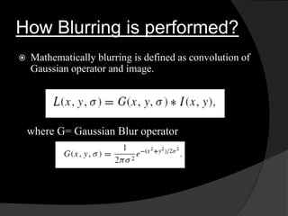
   Mathematically blurring is defined as convolution of
    Gaussian operator and image.


    where G= Gaussian Blur operator
 L is a blurred image
 G is the Gaussian Blur operator
 I is an image
 x, y are the location coordinates
 σ is the “scale” parameter. The amount of
  blur. Greater the value, greater the blur.
 The * is the convolution operation in x and y.
  It applies Gaussian blur G onto the image I
2. Difference of Gaussian(DoG)
 LoG are obtained by taking second order
  derivative.
 DoG images are equivalent to Laplacian of
  Gaussian image. Moreover DoG are scale
  invariant.
 In other word when we do difference of
  gaussian images, it is multiplied with σ2
  which is present in gaussian blur operator G.
3. Finding Keypoint
   Finding keypoint is a two step process:
    1. Locate maxima/minima in DoG images
    2. Find subpixel maxima/minima
Locate maxima/minima

 In the image X is current pixel, while green
  circles are its neighbors, X is marked as
  Keypoint if it is greatest or east of all 26
  neighboring pixels.
 First and last scale are not checked for
  keypoints as there are not enough neighbors
  to compare.
Find subpixel maxima/minima

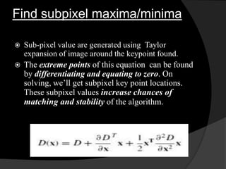
 Sub-pixel value are generated using Taylor
  expansion of image around the keypoint found.
 The extreme points of this equation can be found
  by differentiating and equating to zero. On
  solving, we’ll get subpixel key point locations.
  These subpixel values increase chances of
  matching and stability of the algorithm.
4. Eliminating bad keypoints
1.       Removing Low Contrast features
      If magnitude of intensity at current pixel is less
         than certain value then it is rejected.
2.       Removing edges
         For poorly defined peaks in the DoG
          function, the principal curvature across the edge
          would be much larger than the principal
          curvature along it
         To determine edges Hessian matrix is used.
Tr (H) = Dxx + Dyy
Det(H) = DxxDyy - (Dxy )2


   If the value of R is greater for a candidate
    keypoint, then that keypoint is poorly localized and
    hence rejected.
5. Assigning Orientation
 Gradient direction and magnitude around
  keypoints are collected, and prominent
  orientations are assigned to keypoints.
 Calculations are done relative to this
  orientation, hence it ensure rotation
  invariance.
   The magnitude and orientation is calculated for
    all pixels around the keypoint.
    Then, A histogram is created for this.


   So, orientation can split up one keypoint into
    multiple keypoints
6. Generating SIFT Features
  Creating fingerprint for each keypoint, so that
   we can distinguish between different keypoints.
  A 16 x 16 window is taken around
   keypoint, and it is divided into 16 4 x 4
   windows.
Generating SIFT Features
   Within each 4×4 window, gradient magnitudes
    and orientations are calculated. These
    orientations are put into an 8
    bin histogram, depending on gradient directions.
Generating SIFT Features
 The value added to bin also depend upon distance
  from keypoint ,so gradients which are far are less in
  magnitude.
 This is achieved by using Gaussian weighting
  function.
SIFT
   This has to be repeated for all 16 4x4 regions so
    we will get total 16x8=128 numbers. These 128
    numbers are normalized and resultant 128 numbers
    form feature vector which determine a keypoint
    uniquely.
Problem associated with feature vector
1. Rotation Dependence
   If we rotate the image all the gradient orientation will
    get change. So to avoid this keypoint’s rotation is
    subtracted from each gradient orientation. Hence
    each gradient orientation is relative to keypoint’s
    orientation.
 2. Illumination Dependence
   If we threshold numbers that are big, we can achieve
    illumination independence. So, any number (of the
    128) greater than 0.2 is changed to 0.2. This resultant
    feature vector is normalized again. And now we have
    an illumination independent feature vector.
Application
   Application of SIFT include object
    recognition, gesture recognition, image
    stitching, 3D modeling.
Object recognition
Image
Stitching
References
   http://www.aishack.in/2010/05/sift-scale-invariant-
    feature-transform
   http://en.wikipedia.org/wiki/Scale-invariant feature
    transform
   yumeng-SIFTreport-5.18_bpt.pdf
   Paper on SIFT by Harri Auvinen, Tapio
    Lepp¨alampi, Joni Taipale and Maria Teplykh.
   David G. Lowe, Distinctive Image Features from
    Scale-Invariant Keypoints, International Journal of
    Computer Vision, 2004

More Related Content

SIFT

  • 2. Outline  Introduction to SIFT  Overview of Algorithm  Construction of Scale space  DoG (Difference of Gaussian Images)  Finding Keypoint  Getting Rid of Bad Keypoint  Assigning an orientation to keypoints  Generate SIFT features
  • 3. Introduction to SIFT  Scale-invariant feature transform (or SIFT) is an algorithm in computer vision to detect and describe local features in images.  This algorithm was published by David Lowe.
  • 4. Types of invariance  Illumination
  • 5. Types of invariance  Illumination  Scale
  • 6. Types of invariance  Illumination  Scale  Rotation
  • 7. Types of invariance  Illumination  Scale  Rotation  Full perspective
  • 9. 1. Constructing Scale space  In scale Space we take the image and generate progressively blurred out images, then resize the original image to half and generate blurred images.  Images that are of same size but different scale are called octaves.
  • 10. How Blurring is performed?  Mathematically blurring is defined as convolution of Gaussian operator and image. where G= Gaussian Blur operator
  • 11.  L is a blurred image  G is the Gaussian Blur operator  I is an image  x, y are the location coordinates  σ is the “scale” parameter. The amount of blur. Greater the value, greater the blur.  The * is the convolution operation in x and y. It applies Gaussian blur G onto the image I
  • 12. 2. Difference of Gaussian(DoG)
  • 13.  LoG are obtained by taking second order derivative.  DoG images are equivalent to Laplacian of Gaussian image. Moreover DoG are scale invariant.  In other word when we do difference of gaussian images, it is multiplied with σ2 which is present in gaussian blur operator G.
  • 14. 3. Finding Keypoint  Finding keypoint is a two step process: 1. Locate maxima/minima in DoG images 2. Find subpixel maxima/minima
  • 15. Locate maxima/minima  In the image X is current pixel, while green circles are its neighbors, X is marked as Keypoint if it is greatest or east of all 26 neighboring pixels.  First and last scale are not checked for keypoints as there are not enough neighbors to compare.
  • 16. Find subpixel maxima/minima  Sub-pixel value are generated using Taylor expansion of image around the keypoint found.  The extreme points of this equation can be found by differentiating and equating to zero. On solving, we’ll get subpixel key point locations. These subpixel values increase chances of matching and stability of the algorithm.
  • 17. 4. Eliminating bad keypoints 1. Removing Low Contrast features  If magnitude of intensity at current pixel is less than certain value then it is rejected. 2. Removing edges  For poorly defined peaks in the DoG function, the principal curvature across the edge would be much larger than the principal curvature along it  To determine edges Hessian matrix is used.
  • 18. Tr (H) = Dxx + Dyy Det(H) = DxxDyy - (Dxy )2  If the value of R is greater for a candidate keypoint, then that keypoint is poorly localized and hence rejected.
  • 19. 5. Assigning Orientation  Gradient direction and magnitude around keypoints are collected, and prominent orientations are assigned to keypoints.  Calculations are done relative to this orientation, hence it ensure rotation invariance.
  • 20. The magnitude and orientation is calculated for all pixels around the keypoint. Then, A histogram is created for this.  So, orientation can split up one keypoint into multiple keypoints
  • 21. 6. Generating SIFT Features  Creating fingerprint for each keypoint, so that we can distinguish between different keypoints.  A 16 x 16 window is taken around keypoint, and it is divided into 16 4 x 4 windows.
  • 22. Generating SIFT Features  Within each 4×4 window, gradient magnitudes and orientations are calculated. These orientations are put into an 8 bin histogram, depending on gradient directions.
  • 23. Generating SIFT Features  The value added to bin also depend upon distance from keypoint ,so gradients which are far are less in magnitude.  This is achieved by using Gaussian weighting function.
  • 25. This has to be repeated for all 16 4x4 regions so we will get total 16x8=128 numbers. These 128 numbers are normalized and resultant 128 numbers form feature vector which determine a keypoint uniquely.
  • 26. Problem associated with feature vector 1. Rotation Dependence  If we rotate the image all the gradient orientation will get change. So to avoid this keypoint’s rotation is subtracted from each gradient orientation. Hence each gradient orientation is relative to keypoint’s orientation. 2. Illumination Dependence  If we threshold numbers that are big, we can achieve illumination independence. So, any number (of the 128) greater than 0.2 is changed to 0.2. This resultant feature vector is normalized again. And now we have an illumination independent feature vector.
  • 27. Application  Application of SIFT include object recognition, gesture recognition, image stitching, 3D modeling.
  • 30. References  http://www.aishack.in/2010/05/sift-scale-invariant- feature-transform  http://en.wikipedia.org/wiki/Scale-invariant feature transform  yumeng-SIFTreport-5.18_bpt.pdf  Paper on SIFT by Harri Auvinen, Tapio Lepp¨alampi, Joni Taipale and Maria Teplykh.  David G. Lowe, Distinctive Image Features from Scale-Invariant Keypoints, International Journal of Computer Vision, 2004