Googlevis examples

googleVisExamples
Prepared: VOLKAN OBAN
Reference:https://cran.r-project.org/web/packages/googleVis/vignettes/googleVis_examples.html

GoogleVis:
The googleVis package provides an interface between R and the Google Chart Tools. The functions
of the package allow the user to visualize data stored in R
Installation:
install.packages('googleVis')
library(googleVis)
Bring Your Data to Life with googleVis and R.

First Example
df=data.frame(country=c("US", "GB", "BR"), + val1=c(10,13,14), + val2=c(23,12,32))
Line <- gvisLineChart(df)
plot(Line)

2.Example:
Bar <- gvisBarChart(df)
plot(Bar)

3.Example:
Area <- gvisAreaChart(df)
plot(Area)

4.Example:
SteppedArea <- gvisSteppedAreaChart(df, xvar="country", yvar=c("val1",
"val2"), options=list(isStacked=TRUE))
plot(SteppedArea)

5.Example:
Bubble <- gvisBubbleChart(Fruits, idvar="Fruit", xvar="Sales",
yvar="Expenses", colorvar="Year", sizevar="Profit", options=list(
hAxis='{minValue:75, maxValue:125}'))
plot(Bubble)

6.Example:
M <- matrix(nrow=6,ncol=6) M[col(M)==row(M)] <- 1:6 dat <- data.frame(X=1:6, M)
SC <- gvisScatterChart(dat, options=list( title="Customizing points", legend="right",
pointSize=30, series="{ 0: { pointShape: 'circle' }, 1: { pointShape: 'triangle' }, 2: {
pointShape: 'square' }, 3: { pointShape: 'diamond' }, 4: { pointShape: 'star' }, 5: {
pointShape: 'polygon' } }"))
plot(SC)

7.Example:
Candle <- gvisCandlestickChart(OpenClose, options=list(legend='none'))
plot(Candle)

8.Example:
Gauge <- gvisGauge(CityPopularity, options=list(min=0, max=800, greenFrom=500,
greenTo=800, yellowFrom=300, yellowTo=500, redFrom=0, redTo=300, width=400,
height=300))
plot(Gauge)

9.Example:
Intensity <- gvisIntensityMap(df)
plot(Intensity)

10.Example:
Geo=gvisGeoChart(Exports, locationvar="Country", colorvar="Profit",
options=list(projection="kavrayskiy-vii"))
plot(Geo)

11.Example:
require(datasets)
states <- data.frame(state.name, state.x77)
GeoStates <- gvisGeoChart(states, "state.name", "Illiteracy", options=list(region="US", displayMode="regions", resolution="provinces",
width=600, height=400))
plot(GeoStates)

12.Example:
GeoMarker <- gvisGeoChart(Andrew, "LatLong", sizevar='Speed_kt',
colorvar="Pressure_mb", options=list(region="US"))
plot(GeoMarker)

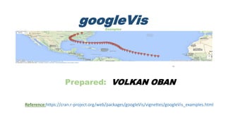
13.Example:
AndrewMap <- gvisMap(Andrew, "LatLong" , "Tip",
options=list(showTip=TRUE, showLine=TRUE, enableScrollWheel=TRUE,
mapType='terrain', useMapTypeControl=TRUE)
plot(AndrewMap)

14.Example:
PopTable <- gvisTable(Population, formats=list(Population="#,###", '% of World
Population'='#.#%'), options=list(page='enable'))
plot(PopTable)

15.Example:
Org <- gvisOrgChart(Regions, options=list(width=600, height=250, size='large',
allowCollapse=TRUE))
plot(Org)

16.Example:
Anno <- gvisAnnotationChart(Stock, datevar="Date", numvar="Value",
idvar="Device", titlevar="Title", annotationvar="Annotation", options=list(
width=600, height=350, fill=10, displayExactValues=TRUE,
colors="['#0000ff','#00ff00']")
plot(Anno)

17.Example:
datSK <- data.frame(From=c(rep("A",3), rep("B", 3)), To=c(rep(c("X", "Y", "Z"),2)),
Weight=c(5,7,6,2,9,4))
Sankey <- gvisSankey(datSK, from="From", to="To", weight="Weight", options=list( sankey="{link:
{color: { fill: '#d799ae' } }, node: { color: { fill: '#a61d4c' }, label: { color: '#871b47' } }}"))
plot(Sankey)

18.Example:
Cal <- gvisCalendar(Cairo, datevar="Date", numvar="Temp", options=list( title="Daily temperature in
Cairo", height=320, calendar="{yearLabel: { fontName: 'Times-Roman', fontSize: 32, color:
'#1A8763', bold: true}, cellSize: 10, cellColor: { stroke: 'red', strokeOpacity: 0.2 }, focusedCellColor:
{stroke:'red'}}") )
plot(Cal)

19.Example:
datTL <- data.frame(Position=c(rep("President", 3), rep("Vice", 3)), Name=c("Washington", "Adams",
"Jefferson", "Adams", "Jefferson", "Burr"), start=as.Date(x=rep(c("1789-03-29", "1797-02-03", "1801-02-
03"),2)), end=as.Date(x=rep(c("1797-02-03", "1801-02-03", "1809-02-03"),2)))
Timeline <- gvisTimeline(data=datTL, rowlabel="Name", barlabel="Position", start="start", end="end",
options=list(timeline="{groupByRowLabel:false}", backgroundColor='#ffd', height=350, colors="['#cbb69d',
'#603913', '#c69c6e']"))
plot(Timeline)

20.Example:
G <- gvisGeoChart(Exports, "Country", "Profit", options=list(width=300, height=300))
T <- gvisTable(Exports, options=list(width=220, height=300))
GT <- gvisMerge(G,T, horizontal=TRUE)
plot(GT)

21.Example:
Motion=gvisMotionChart(Fruits, idvar="Fruit", timevar="Year")
plot(Motion)

22.Example:
AndrewGeo <- gvisGeoMap(Andrew, locationvar="LatLong", numvar="Speed_kt",
hovervar="Category", options=list(height=350, region="US", dataMode="markers"))
plot(AndrewGeo)

23.Example:
AnnoTimeLine <- gvisAnnotatedTimeLine(Stock, datevar="Date", numvar="Value", idvar="Device",
titlevar="Title", annotationvar="Annotation", options=list(displayAnnotations=TRUE,
width="600px", height="350px"))
plot(AnnoTimeLine)

Googlevis examples

More Related Content

Googlevis examples