A Multiple-Shooting Differential Dynamic Programming Algorithm
- 1. A Multiple-Shooting Differential Dynamic Programming Algorithm Etienne Pellegrini Ryan P. Russell 27th Spaceflight Mechanics Meeting, San Antonio, TX 02/06/2017
- 2. Summary • Introduction and Background • Multiple-Shooting Problem Formulation • Solving the multiple-shooting problem - Augmented Lagrangian methods - Single-leg expansions - Multi-leg expansions • Numerical results - Validation of the quadratic expansions and updates - Van Der Pol Oscillator - 2D Spacecraft Orbit Transfer • Conclusions and future work 2
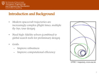
- 3. Introduction and Background • Modern spacecraft trajectories are increasingly complex (flight times, multiple fly-bys, tour design) • Need high-fidelity solvers (combined to global search tools for preliminary design) • Goals: - Improve robustness - Improve computational efficiency GTOC 1 trajectory, www.esa.int 3
- 4. Motivations • Multi-phase capabilities: - Separation at flybys, interception, rendez-vous, etc… - Each phase can have different dynamics, constraints, etc… • Multi-shooting framework: - Allows for the decoupling of the legs and phases - Reduces sensitivities and improves robustness - Parallel implementation (solving each leg independently). 4
- 5. Hybrid Differential Dynamic Programming Classic NLP Solvers DDP Methods 5
- 6. Summary • Introduction and Background • Multiple-Shooting Problem Formulation • Solving the multiple-shooting problem - Augmented Lagrangian methods - Single-leg expansions - Multi-leg expansions • Numerical results - Validation of the quadratic expansions and updates - Van Der Pol Oscillator - 2D Spacecraft Orbit Transfer • Conclusions and future work 6
- 8. The Multi-Shooting Subinterval: the Legs 8
- 11. Summary • Introduction and Background • Multiple-Shooting Problem Formulation • Solving the multiple-shooting problem - Augmented Lagrangian methods - Single-leg expansions - Multi-leg expansions • Numerical results - Validation of the quadratic expansions and updates - Van Der Pol Oscillator - 2D Spacecraft Orbit Transfer • Conclusions and future work 11
- 12. • Mixed approach: - Box constraints on the state or controls - “Hard’’ constraints, can not be violated to first order by the update laws - Accounted for using constrained quadratic programming - In MDDP as it is, using a null-space method in the TR algorithm - Terminal constraints (intra- and inter-phase) and path constraints - Accounted for using an augmented Lagrangian technique Handling the constraints 12
- 13. The Augmented Lagrangian Algorithm • Penalization method for constrained optimization • Transforms a constrained problem into an unconstrained one by adding a penalty and Lagrange multipliers to the cost function: 13
- 18. Inner Loop of the MS Algorithm 18
- 20. The MDDP Algorithm with AL 20
- 21. Summary • Introduction and Background • Multiple-Shooting Problem Formulation • Solving the multiple-shooting problem - Augmented Lagrangian methods - Single-leg expansions - Multi-leg expansions • Numerical results - Validation of the quadratic expansions and updates - Van Der Pol Oscillator - 2D Spacecraft Orbit Transfer • Conclusions and future work 21
- 22. Validation and Numerical Results • Validation of the quadratic expansions and updates is done using a quadratic problem with linear constraints: 22
- 23. Linear Quadratic Problem Initial States Final States Controls 23
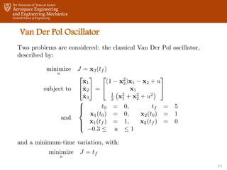
- 24. Van Der Pol Oscillator 24
- 25. Classical VDP Final State Controls 25
- 26. Minimum-Time VDP Final State Controls 26
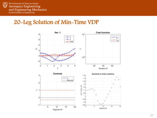
- 27. 20-Leg Solution of Min-Time VDP 27
- 28. 2D Spacecraft Orbit Transfer 28
- 29. 2DSpacecraft Solution Initial State Final State Controls 29
- 32. Conclusions & Future work • The theoretical developments necessary to the formulation of a multiple-shooting differential dynamic programming algorithm are presented for the first time. • An algorithm based on augmented Lagrangian methods and multiple-shooting DDP is described and tested, allowing to confirm: - The validity of the quadratic expansions and update equations - The applicability of the multiple-shooting principles to DDP - The resulting reduction in sensitivity for the subproblems • Future work: - Parallel implementation - Robustness and performance analysis on more complex test problems 32
- 34. References (I) • D. Rufer, “Trajectory Optimization by Making Use of the Closed Solution of Constant Thrust- Acceleration Motion,” Celestial Mechanics, Vol. 14, No. 1, 1976, pp. 91–103. • C. H. Yam, D. Izzo, and F. Biscani, “Towards a High Fidelity Direct Transcription Method for Optimisation of Low-Thrust Trajectories,” 4th International Conference on Astrodynamics Tools and Techniques, 2010, pp. 1–7. • G. Lantoine and R. P. Russell, “Complete closed-form solutions of the Stark problem,” Celestial Mechanics and Dynamical Astronomy, Vol. 109, Feb. 2011, pp. 333–366, 10.1007/s10569-010- 9331-1. • R. R. Bate, D. D. Mueller, and J. E. White, Fundamentals of Astrodynamics. New-York, NY. Dover Publications, 1971. • Lyness, J. N. and Moler, C. B., “Numerical Dierentiation of Analytic Functions," SIAM Journal on Numerical Analysis, Vol. 4, No. 2, 1967, pp. 202-210. • Squire, W. and Trapp, G., “Using Complex Variables to Estimate Derivatives of Real Functions,” SIAM Review, Vol. 40, No. 1, Jan 1998, pp. 110-112. • Martins, J. R. R. A., Sturdza, P., and Alonso, J. J., “The Connection Between the Complex-Step Derivative Approximation and Algorithmic Differentiation,” Proceedings of the 39th Aerospace Sciences Meeting and Exhibit, AIAA, Reno, NV, jan 2001. 34
- 35. References (II) • Lantoine, G., Russell, R. P., and Dargent, T., “Using Multicomplex Variables for Automatic Computation of High-Order Derivatives,” ACM Transactions on Mathematical Software, Vol. 38, No. 3, apr 2012, pp. 16:1-16:21. • G. Lantoine and R. P. Russell, “A Hybrid Differential Dynamic Programming Algorithm for Constrained Optimal Control Problems. Part 1: Theory,” Journal of Optimization Theory and Applications, Vol. 154, apr 2012, doi:10.1007/s10957-012-0039-0. • Conn, A.R., Gould, N.I.M., Toint, P.L., Trust-Region Methods. MPS - SIAM, Philadelphia, 2000. • Bellman, R., Dynamic Programming, Princeton University Press, Princeton, New Jersey, 1957. • Davidon, W.C., “Variable Metric Method for Minimization”, SIAM Journal on Optimization, Vol. 1, Issue 1, 1991, pp. 1 - 17. 35
Editor's Notes
- Good morning, and welcome to this research seminar, during which I will present a summary of the research conducted during my doctoral program. I will focus primarily on my latest project, the application of multiple-shooting principles to differential dynamic techniques.
- Today, we’ll start by talking about multiple-shooting in differential dynamic programming. This is the project I’ve worked on in the past year, First, I’ll present some background on the methods we used in this project, and in particular on the HDDP algorithm, which was developed as some of you probably know by Gregory Lantoine and Ryan at Georgia Tech. Then we’ll move on to reformulation of the problem according to multiple-shooting principles. We’ll talk about the structure of the multiple-shooting algorithm, which I call MDDP, and we’ll look at some preliminary results that I obtained with my implementation of MDDP. The second half of the presentation will be dedicated to 3 projects that I worked on during my PhD, and which can all be used in the context of the MDDP algorithm, and of the three main goals of my PhD research
- So, what are we about to see here? The motivation behind my doctoral research is the increasing complexity of modern spacecraft trajectories. The different problems of the well known Global Trajectory Optimization Competition are a good example of the challenges encounters, when optimizing trajectories, such as fly-bys, long flight times, low and continuous thrust, etc… There are three main goals to my PhD research, which are: to improve the robustness of a high-fidelity solver ; to reduce the amount of human effort ; and to improve the computational efficiency of the solver.
- [7.30] So why multiple shooting? Most optimal control problems are formulated with multiple phases, so that the dynamics, cost, constraints can change in time, and to allow us to simulate flybys, separations, etc. The multiple-shooting formulation will allow us to decouple those phases, and even to split them in subintervals, in order to reduce the time interval considered for each subproblem. This reduces sensitivities and should improve robustness. We’ll also see that multiple-shooting has a high potential for parallel implementation
- A high-level view of the difference between a classic NLP solver and a DDP method is this: In direct NLP solvers, the trajectory is discretized and all the unknowns for the whole trajectory are solved for while trying to resepct all of the constraints. This results in usually very large, although sparse problems. In DDP, we split a huge problem into a succession of smaller, easier to solve subproblems, starting at the end of the trajectory and updating backwards. HDDP uses state-transition matrices to propagate the sensitivities backwards and link the subproblems.
- Today, we’ll start by talking about multiple-shooting in differential dynamic programming. This is the project I’ve worked on in the past year, First, I’ll present some background on the methods we used in this project, and in particular on the HDDP algorithm, which was developed as some of you probably know by Gregory Lantoine and Ryan at Georgia Tech. Then we’ll move on to reformulation of the problem according to multiple-shooting principles. We’ll talk about the structure of the multiple-shooting algorithm, which I call MDDP, and we’ll look at some preliminary results that I obtained with my implementation of MDDP. The second half of the presentation will be dedicated to 3 projects that I worked on during my PhD, and which can all be used in the context of the MDDP algorithm, and of the three main goals of my PhD research
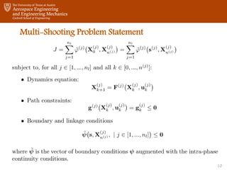
- Ok, now we’re going to get a little more in the nitty-gritty. We start with a general multi-phase optimal control problems. We have our objective function, dynamics equation, paths constraints and boundary conditions. The superscript I in brackets indicates that the quantities are related to phase [i]. Also, in all of the following, we only consider problems of Mayer, with only a terminal cost. If we have an integral cost, we can augment the state vector to transform the problem.
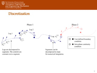
- The multiple phase optimal control problem is already quite amenable to a multiple-shooting formulation, but in order to increase the flexibility on the number of subintervals, we split the phases in legs. The legs within a phase are connected by simple continuity conditions. Moreover, the vector s of multiple-shooting variables is introduced. It’s composed of all the initial conditions of each leg.
- So the discretization looks like this: you have two phases in two different colors here, linked by a user defined boundary condition, those two squares. Then each phase is divided into legs, linked to each other by simple continuity conditions. The legs are split in segments and the thrust is constant on each segment. The X_0s of each leg, here, here, here, form the s vector of multiple-shooting variables.
- Once the discretization is defined, and we’ve assigned the correct dynamics, constraints, boundaries, to each leg, we can write the general problem this way. The objective function is the sum of the cost over each leg, and now depends on the s vector, as well as on the controls. Our approach consists in first solving for the controls over one leg, before updating the initial conditions of each leg.
- Today, we’ll start by talking about multiple-shooting in differential dynamic programming. This is the project I’ve worked on in the past year, First, I’ll present some background on the methods we used in this project, and in particular on the HDDP algorithm, which was developed as some of you probably know by Gregory Lantoine and Ryan at Georgia Tech. Then we’ll move on to reformulation of the problem according to multiple-shooting principles. We’ll talk about the structure of the multiple-shooting algorithm, which I call MDDP, and we’ll look at some preliminary results that I obtained with my implementation of MDDP. The second half of the presentation will be dedicated to 3 projects that I worked on during my PhD, and which can all be used in the context of the MDDP algorithm, and of the three main goals of my PhD research
- But first, how do we handle the constraints? Well we consider two sorts of constraints, according to the philosophy of HDDP. For the sake of simplicity both types were noted using the $g$ and $\psi$ functions in the problem statement. First we have box constraints that we can apply to the controls or to the multiple-shooting variables. These are called “hard” constraints and we use a null-space trust-region method to ensure first-order adherence to the bound. Then we have all the terminal and path constraints, including the new continuity conditions, which are called “soft” constraints and we relax them and use an augmented Lagrangian method to treat them.
- Speaking of which, what is an augmented Lagrangian algorithm? Well it’s a way to use unconstrained optimization methods to solve a constrained problem. We penalize the cost function, adding a penalty term, and Lagrange multipliers. The solutions of the two problems the same if c is greater than a prescribed value, the idea being that if psi is not zero, then d_c will tend to infinity, and if psi is zero, then the problems are equivalent.
- So, how do we put together DDP, multiple-shooting, and augmented Lagrangian? Solve the INNER LOOP problem, with constant lambdas and cs. The idea is to use DDP to solve for the controls, and then to solve for their initial conditions. Start by solving for the controls, using the one-leg problem As I said, we first have to solve the inner loop problem, with constant lambdas and cs We start by solving for the controls for each leg, and for that, we look at the one leg problem, which is easy to extract from the multiple shooting general formulation. And now we’re going to solve for its controls using a modified version of HDDP, that also allows us to obtain sensitivities with respect to the $s$ vector! The maths can be found in the paper that’ll be presented in San Antonio, and I’ll only present the key steps
- Like in HDDP, we start from quadratic expansions of the cost-to-go. We now have extra terms because of the dependence on s The control law also now has a feedback in delta s, to account for changes in the initial conditions of all the other legs. So we use this control law, plug it back in the quadratic expansions, use state-tranition matrices to map the controls free partials backwards, and proceed with our backward sweep, exactly like with HDDP but with extra terms.
- When we get to the end of the backward sweep, we have the following cost expansion for leg j. Which, noting that delta X0 of leg j is delta s\j, we can rewrite it like this (also adding back all the superscript j’s now)
- Then the total cost for the problem is the sum of all the legs costs, we define the cap lambda vector as the concatenation of all the lagrange multipliers for all the legs. Then we can use all the partials that we got from the HDDP iterations on the legs to form the JS, JSS, Jlam, JLAMLAM matrices, and write the cost this way. Then we can minimize with respect to delta s, and obtain the control law that you see here for the update of the initial conditions of the legs! This concludes one iteration of the inner loop. Note that in most iterations, as long as we’re not approximately converged, we don’t update the LMs, and therefore this control law becomes a simple update.
- So this is what our inner loop looks like. We first initialize everything, then we can run the one-leg solver. Note that it can be done in parallel because the legs are independent from each other at this step! The one leg solver is essentially one iteration of the HDDP algorithm, without the LM update. Once all the legs have been optimized in parallel, we use the trust region again as a multi-shooting solver, and update the vector s. We can then test for convergence, and if approximately converged, move on to the LM and penalty update.
- Most augmented lagrangian algorithm use a steepest descent step for the lagrange multipliers update. In MDDP however, we have second order partials of the cost wrt to the lambdas and we can build a second-order update, using the trust-region again.
- This is the general structure of the MDDP algorithm. Once again, after the initialization, we go to the inner loop, iterate on the legs controls and initial conditions until approximately converged. Then we test the constraints feasibility. If the constraints aree completely violated, we crank up the penalty parameter to force the problem to move towards feasibility. If the constraints are almost respected, we update the Lagrange multipliers.
- Today, we’ll start by talking about multiple-shooting in differential dynamic programming. This is the project I’ve worked on in the past year, First, I’ll present some background on the methods we used in this project, and in particular on the HDDP algorithm, which was developed as some of you probably know by Gregory Lantoine and Ryan at Georgia Tech. Then we’ll move on to reformulation of the problem according to multiple-shooting principles. We’ll talk about the structure of the multiple-shooting algorithm, which I call MDDP, and we’ll look at some preliminary results that I obtained with my implementation of MDDP. The second half of the presentation will be dedicated to 3 projects that I worked on during my PhD, and which can all be used in the context of the MDDP algorithm, and of the three main goals of my PhD research
- The first problem I have here I took from Gregory’s HDDP application paper, and used with the same intent, to validate the quadratic expansions and update equations. It’s a quadratic problem with linear constraints, so it should be solved by an augmented lagrangian approach in exactly one iteration.
- And here is the solution of our simple problem. Both the single-shooting and multiple-shooting versions of MDDP converge to the same solution, up to the convergence tolerance. That’ll actually be the case in all of the following slides The real reduction and expected reduction agree to machine precision, the problem converges in one iteration, we’re happy, our quadratic expansions look correct.
- So we move on to a slightly more complicated problem, the classical Van Der Pol oscillator, described here: I’ll also show results with a minimum-time variant of VDP
- Smooth controls, not a difficult problem Here we can see the solution of the classical Van Der Pol oscillator for the constraints listed on the previous slide. The controls are smooth. Note that the cost is not continuous: since it’s an integral cost, we don’t need to make it continuous and we can just add together the costs of all the legs
- The minimum-time Van Der Pol presents the expected bang-bang structure
- Let’s have a look at how MDDP solves this problem with a single-phase and 20 leg. Note once again that the cost is discontinuous. The problem is continuous at first, because the legs are initialized by propagating the phase’s initial conditions. However, pretty quickly, they start separating. Once the penalty parameter starts getting updated, we can see the algorithm going back towards feasibility, trying to make the legs continuous again.The sensitivities are all very small.
- The 2D spacecraft orbit transfer is a variation on a problem from Bryson and Ho. The equations of motion are in polar coordinates, and the controls are the thrust magnitude and the angle of the thrust with respect to the tangential direction. The cost here is the integral of the square of the thrust magnitude, so we won’t get a bang-bang structure, but smooth, quite easy to converge solutions
- Here you can see the initial state, with an initial guess that has a very small thrust in the tangential direction at all times, and the converged solution, going from radius 1 to radius 3. Both single-shooting and multiple-shooting formulations converged to the same solution, up to the convergence tolerance.
- Let’s watch how the single and multiple shooting go to the solution. You can observe then sensitivity to the initial conditions on the bottom right, which is on the order of 80,000, meaning a delta X_0 of 1 distance unit would result in a delta X_final of 80,000 distance units. You can also see the total cost function Jtot including the constraints, which usually decreases at each iteration. It can increase when the penalty parameter is changed or the lagrange multiplers
- In the multiple shooting version, with 1 legs, the maximum sensitivities are divided by about 60, which is what we expect from multplie shooting. In this particular case, there is no evidence of any benefits of the ms on the efficiency of the algorithm, since it takes a few more iterations. I’m working at the moment on a comparative study of the robustness and efficiency of the single vs multiple shooting, and hope to publish an application paper in the next few months.
