Brock Butlett Time Series-Great Lakes

Great Lakes Annual Precipitation, 1900-1986
Brock Butlett
March 21, 2017
Abstract.
An analysis of the annual precipitation of rainfall in inches over the entire Great Lakes area,
Michigan. The experiment uses the "Box-Jenkins Methodology" to fit an autoregressive
integrated moving average model ARIMA(p,d,q) to the given time series, for the purpose of
forecasting future levels of precipitation. The "Box-Jenkins Methodology" requires a
stationary series that accounts for any seasonality present in the data. This approach
identifies the best ARMA model(s) to select when constructing the model.
The "Great Lakes" data set is an example of a non-seasonal, non-stationary time series that
experiences a slight upward linear trend. The series is differenced and transformed using
"Box-Cox" in order to stabilize the mean and variance, correcting for stationarity. The best
model fitted for the data was an ARIMA(4,1,0) found by observing the partial and auto
correlation functions. The fit suggested the best estimates for the coefficients via the AIC.
Verified as independent random variables, the residuals of the fitted model were tested for
normality using the McLeod-Li, Ljung-Box, and Shapiro-Wilk test. The model proved to be
an adequate representation of the data providing reasonable predictions for precipitation.
Introduction.
A study of the Annual rainfall in the surrounding Great Lakes area in Michigan. Data was
collected from 1900-1986 and documented as a series of successive values courtesy of
Prof. Rob Hyndman's Time Series Data Library. For the given series, I would like to capture
a model to accurately predict the annual levels of precipitation and diagram the projected
totals for the next 5 years. I am motivated in this particular set not only because it is a well
documented area, but also to provide as a general starting point for studying variations in
weather and changes in climate. I eventually want to be able to apply this skill to different
aspects of weather, specifically forecasting natural disasters and other extreme systems.

Original Plot.
• Trend: There does seem to be a slight upward linear trend of the data. That seems to
be potentially growing over time.
• Seasonality: Considering the data is recorded annually, and there is no apparent
pattern visible throughout the data. we will conclude the data does not have a seasonal
component, the plots being quite random in structure.
• Behavior: The overall senses of the data set seems to take a consistent extreme
high/low behavior; but nothing that sticks out as inconsistent relative to the rest of the
data set. Had the series been a bit more inconsistent with sharp behavior the "Box-
Jenkins" approach may not not work here and the behavior could suggest just a
"Random Walk" where the series is just completely random over time.
Box Cox Transformation.
Here we are interested in stabilizing variance and transforming the data to replicate a
normal distribution. In order to do this we choose lambda that maximizes the likelihood for
the data and apply the transformation to our series.
𝜆 =
𝑋𝑡 − 1
𝜆
𝜆 = 𝑙𝑜𝑔(𝑋𝑡)
when 𝜆 > 0 or 𝑙𝑎𝑚𝑏𝑑𝑎 = 0 respectively.

The lambda that will best transform our data is one that maximizes the likelihood. Notice in
the graph above the lambda inside our 95% confidence interval that does is nearly zero.
Thus we will use a log transformation to stabilize the variance within the series
Differencing.
• Removing Trend: In order to remove trend we must difference the data by taking
𝑋𝑡 − 𝑋𝑡−1. This removes the upward linear trend in the series and centers the mean
around zero. Pictured in the graph above.
Over Differencing.
Sometimes it is necessary to difference a series twice to correct for trend within the data.
This happens when the time series takes a quadratic form instead of a linear one. In the
original plot of "Great Lakes" series the data seemed to take a possible increasing quadratic
form.

• Increasing Variance: Notice at first glance, differencing the series twice the plot
seemed to tighten up around zero for a seemingly better fit. Yet the problem lies with
increasing variance. Comparing the approaches, differencing once had a Variance of
0.01258 , while differencing twice and a variance of 0.03896. The jump is a key sign of
over differencing, and model represents more of a linear than quaratic form.
Identifying the model.
In order to identify and select the correct model we must look at the partial and auto
correlation functions. Here is a look at the ACF and PACF of the original time series
The ACF of the original time series does not show much here, the series resembles a
"random walk" which cannot be modeled or a possible Moving average MA(5). The original
series is not stationary
Let’s take at the ACF and PACF after transforming and differencing the series. After
stabilizing the mean and variance, removing the trend in the data.

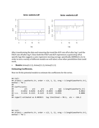
After transforming the data and removing the trend the ACF cuts off at after lag 1 and the
PACF cuts off after lag 4. Since both the PACF and ACF experiences a quick drop off at
specific lags this suggests a auto regressive moving average. specifically ARIMA(4,1,1). In
order to test a variety of different models we will select a few other possibilities that could
work.
• Models Arima(4,1,1), Arima(2,1,1), Arima(3,1,1)
Estimating Coefficients.
Now we fit the potential models to estimate the coefficients for the series.
## Call:
## arima(x = weatherts.tr, order = c(4, 1, 1), xreg = 1:length(weatherts.tr),
method = "ML")
##
## Coefficients:
## ar1 ar2 ar3 ar4 ma1 1:length(weatherts.tr)
## -0.0452 0.0296 -0.0272 -0.0493 -1.0000 0.0012
## s.e. 0.1116 0.1115 0.1125 0.1119 0.0391 0.0004
##
## sigma^2 estimated as 0.005813: log likelihood = 90.1, aic = -166.2
## Call:
method = "ML")

##
## Coefficients:
## ar1 ar2 ma1 1:length(weatherts.tr)
## -0.0431 0.0312 -1.0000 0.0012
## s.e. 0.1119 0.1115 0.0377 0.0004
##
## Call:
method = "ML")
##
## Coefficients:
## ar1 ar2 ar3 ma1 1:length(weatherts.tr)
## -0.0428 0.0294 -0.0233 -1.0000 0.0012
## s.e. 0.1118 0.1117 0.1125 0.0381 0.0004
##
## sigma^2 estimated as 0.005835: log likelihood = 90, aic = -168
Notice for our proposed model of Arima(4,1,1) does have the AIC closest to zero (AIC = -
166.2 ) which suggests this is our best model. Yet one thing to pay attention to is the
estimated coefficient of the Moving average component is exactly -1. This means the
ARIMA(4,1,1) model is not stationary and falls out of the desired [-1,1] range after
accounting for the standard deviation of 0.0391.
We will try to correct this by excluding the moving average component in our proposed
model and use ARIMA(4,1,0) or ARIMA(2,1,0) as our new potential model.
## Call:
## Coefficients:
## ar1 ar2 ar3 ar4 1:length(weatherts.tr)
## -0.8600 -0.6464 -0.4965 -0.3592 0.0010
## s.e. 0.1044 0.1310 0.1290 0.1042 0.0027
##
## Call:
method = "ML")
##
## Coefficients:
## ar1 ar2 1:length(weatherts.tr)
## -0.7044 -0.3134 9e-04
## s.e. 0.1061 0.1057 5e-03
Now we have two models where all the coefficients lie within the desired range, the AIC is
lower, and now the proposed models are stationary.

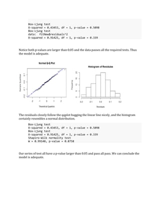
We will narrow are attention to these two models. With Arima(2,1,0) ranking as our best
model and ARIMA(4,1,0) as secondary.
• Model: ARIMA(p,d,q)
𝑋𝑡 = 𝜙1 𝑋𝑡−1 + 𝜙2 𝑋𝑡−2 − +. . . +𝜙 𝑝 𝑋𝑡−𝑝 − 𝜃1 𝑎 𝑡−1 − 𝜃2 𝑎 𝑡−2. . . −𝜃𝑞𝑎 𝑡−𝑎
Diagnostic Checking.
In order to use these model with any faith we must verify the model is adequate. We will do
this by checking if the residuals are randomly distributed and follow a normal distribution.
1.Are the Residuals normally distributed?
• Check if the residuals follow the qqnorm() plot
• Do residuals resemble a normal curve
Looking at the results above the residuals relatively hug the linear line and the histogram
has a resemblance to the normal distribution.
To verify results above we will use the Shapiro-Wilk test to check for normality.
Shapiro-Wilk normality test
W = 0.99148, p-value = 0.8758
Our p-value is larger than our testing level of $ = 0.05 $ so we can conclude the data came
from a normal distribution.
Finally we must check to see if the autocorrelations of the time series are different from
zero. Which would imply the observed correlations in the data are just a result of the
sampling process. To do this we will use the Ljung-Box, and McLeod-Li test: (Note: McLeod-
Li test checks the Ljung-Box squares)

Box-Ljung test
X-squared = 0.43453, df = 1, p-value = 0.5098
Box-Ljung test
data: fitNew$residuals^2
Notice both p-values are larger than 0.05 and the data passes all the required tests. Thus
the model is adequate.
The residuals closely follow the qqplot hugging the linear line nicely, and the histogram
certainly resembles a normal distribution.
Box-Ljung test
Box-Ljung test
Shapiro-Wilk normality test
W = 0.99148, p-value = 0.8758
Our series of test all have a p-value larger than 0.05 and pass all pass. We can conclude the
model is adequate.

Forecasting.
Now that we have gone through all of the steps of selecting models and verifying that they
are adequate representation of the data. We will use them to forecast future levels of rain
fall in the surrounding Great lakes area and check if the predictions are reasonable. Our
95% confidence intervals should capture the entirety of possibilities the data may take on
in order to conclude positive results.
To do this I have removed the data entries for the years 1981-1986 from the original series
and will check how accurate the 5 forecasted totals coincide with the actual true rainfall
totals for the corresponding years.
ARIMA(2,1,0):
The model seems to accurately forecast reasonable levels of rainfall but the the 95%
confidence interval doesnt capture the spike at 1985 where it jumps to 40inches of rainfall.
The model may not be a good a good choice. Also the projected totals seem to lack any type
of spikes in behavior and tends to follow more of a straight behavior. This goes against the
grain of all the past totals through the series.

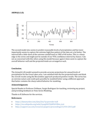
ARIMA(4,1,0):
The second model also seems to predict reasonable levels of precipitation and but more
importantly seems to capture the extreme high/low pattern of the data set a lot better. The
interval falls a little short of the extreme rainfall total at 1985 of 40 inches. This is a sharp
edge in the series and might just lie outside of our 95% confidence interval by chance. I am
not as concerned with this when using this model because again it does seem to capture the
overall behavior well and the projected totals are arranged as such.
Conclusion.
The Arima(4,1,0) model seemed to provide accurate projections for annual levels of
precipitation for the Great Lakes area. I am satisfied with the five projected totals and think
the overall results using the Box Jenkins approach produced positive results. The series has
an extreme nature and could quite possibly be modeled better using a different approach
that better contains the sharp radical behavior for modeling.
Acknowledgments
Special thanks to Professor Feldman, Sergio Rodriguez for teaching, reviewing my project,
and providing feedback on Time Series Modeling.
Thanks to R Software for the services.
References:
• https://datamarket.com/data/list/?q=provider:tsdl
• https://en.wikipedia.org/wiki/Ljung%E2%80%93Box_test
• http://support.sas.com/resources/papers/proceedings13/454-2013.pdf

Appendix:
dataWeather = read.csv("C:UsersBrockDesktopweather.orig.txt")
weatherts = ts(dataWeather$X31.6)
plot(weatherts)
var(weatherts)
acf(weatherts)
pacf(weatherts)
# Model: Arima(0,0,5)
#increasing variance box cox transformation
bctransform <- boxcox(dataWeather$X31.69 ~as.numeric(1:length(dataWeather$X31
.69)))
bctransform$x[which(bctransform$y == max(bctransform$y))]
#transformation
weatherts.tr = log(weatherts)
plot(weatherts.tr)
#differncing to remove upward trend
weatherts.tr.diff = diff(weatherts.tr)
plot(weatherts.tr.diff)
var(weatherts.tr.diff)
abline(h = 0.2, col = 'red')
abline(h = -0.2, col ='red')
abline(h = 0, col = 'blue')
#over differencing variance spiked de-stablizes
weatherts.tr.diff2 = diff(weatherts.tr,differences = 2)
plot(weatherts.tr.diff)
var(weatherts.tr.diff2)
abline(h = 0.2, col = 'red')
abline(h = -0.2, col ='red')
abline(h = 0, col = 'blue')
#acf pacf of new tr.diff
acf(weatherts.tr.diff)
pacf(weatherts.tr.diff)
# Model: Arima(4,1,1), Arima(2,1,1), Arima(3,1,1), Arima(4,1,0)
#suggested
arima(weatherts.tr, order = c(4,1,1), method = "CSS")

# my fits, fit 2 and 3 are good, Fit2 is best.
fit1 = arima(weatherts.tr, order = c(0,0,5), method = "ML",xreg=1 : length(w
eatherts.tr))
eatherts.tr))
eatherts.tr))
eatherts.tr))
#fit 2 diagnostics
qqnorm(fit2$residuals)
qqline(fit2$residuals, col ='blue')
hist(fit2$residuals, xlab = "Residuals" , main = "Histogram of Residulas")
resid.ts = (fit2$residuals)
plot(resid.ts)
abline(lm(resid.ts ~ as.numeric(1:length(resid.ts))))
abline(h=mean(resid.ts), col="red")
mean(resid.ts)
var(resid.ts)
Box.test(fit2$residuals, lag = 1, type = "Ljung-Box")
Box.test(fit2$residuals^2, lag = 1, type = "Ljung-Box")
shapiro.test(fit2$residuals)
#fit 3 diagnostics
qqnorm(fit4$residuals)
qqline(fit4$residuals, col ='blue')
hist(fit4$residuals, xlab = "Residuals" , main = "Histogram of Residulas")
resid.ts = (fit4$residuals)
plot(resid.ts)
abline(lm(resid.ts ~ as.numeric(1:length(resid.ts))))
abline(h=mean(resid.ts), col="red")
mean(resid.ts)
var(resid.ts)

Box.test(fit4$residuals, lag = 1, type = "Ljung-Box")
Box.test(fit4$residuals^2, lag = 1, type = "Ljung-Box")
shapiro.test(fit4$residuals)
# predicting with fit 2
pred <- predict(fit2, n.ahead = 5, newxreg=(length(weatherts.tr)+1) : length(
weatherts.tr)+5)
pred.orig = exp(pred$pred)
pred.se = exp(2*pred$pred*pred$se)
ts.plot(dataWeather$X31.69, xlim=c(1,length(dataWeather$X31.69)+5), ylim = c(
25,max(pred.orig+1.96*pred.se+5)))
points((length(dataWeather$X31.69)+1):(length(dataWeather$X31.69)+5),pred.ori
g, col="red")
lines((length(dataWeather$X31.69)+1):(length(dataWeather$X31.69)+5),pred.orig
+1.96*pred.se,lty=2, col="blue")
-1.96*pred.se,lty=2, col="blue")
#predicting with fit 3
pred <- predict(fit3, n.ahead = 5, newxreg=(length(weatherts.tr)+1) : length(
weatherts.tr)+5)
pred.orig = exp(pred$pred)
pred.se = exp(2*pred$pred*pred$se)
ts.plot(dataWeather$X31.69, xlim=c(1,length(dataWeather$X31.69)+5), ylim = c(
25,max(pred.orig+1.96*pred.se+5)))
points((length(dataWeather$X31.69)+1):(length(dataWeather$X31.69)+5),pred.ori
g, col="red")
+1.96*pred.se,lty=2, col="blue")
-1.96*pred.se,lty=2, col="blue")

Brock Butlett Time Series-Great Lakes

More Related Content

Brock Butlett Time Series-Great Lakes