classification in data warehouse and mining

2
 Classification
 Predicts categorical class labels (discrete or nominal)
 Classifies data (constructs a model) based on the training set
and the values (class labels) in a classifying attribute and
uses it in classifying new data.
 For example, we can build a classification model to
categorize bank loan applications as either safe or risky.
 Prediction
 models continuous-valued functions, i.e., predicts unknown
or missing values
 Typical applications
 Credit approval
 Target marketing
Classification vs. Prediction

3
Classification—A Two-Step Process
 Data classification is a two-step process:
 Learning step (where a classification model is constructed)
 Classification step (where the model is used to predict class
labels for given data).
 In the learning step (or training phase), a classification algorithm
builds the classifier by analyzing or “learning from” a training set.
 A tuple, X, is represented by an N-dimensional attribute vector,
X ={x1, x2,……..xN}
 Each tuple, X, is assumed to belong to a predefined class as
determined by another database attribute called the class label
attribute.
 The individual tuples making up the training set are referred to as
training tuples and are randomly sampled from the database under
analysis.

6
Process (1): Model Construction
Training
Data
NAME RANK YEARS TENURED
Mike Assistant Prof 3 no
Mary Assistant Prof 7 yes
Bill Professor 2 yes
Jim Associate Prof 7 yes
Dave Assistant Prof 6 no
Anne Associate Prof 3 no
Classification
Algorithms
IF rank = ‘professor’
OR years > 6
THEN tenured = ‘yes’
Classifier
(Model)

7
Process (2): Using the Model in Prediction
Classifier
Testing
Data
NAME RANK YEARS TENURED
Tom Assistant Prof 2 no
Merlisa Associate Prof 6 no
George Professor 5 yes
Joseph Assistant Prof 7 yes
Unseen Data
(Jeff, Professor, 4)
Tenured?

8
Supervised vs. Unsupervised Learning
 Supervised learning (classification)
 Supervision: The training data (observations,
measurements, etc.) are accompanied by labels indicating
the class of the observations
 New data is classified based on the training set
 Unsupervised learning (clustering)
 The class labels of training data is unknown
 In this we can predict the class labels by using clustering
technique.

Issues regarding
Classification & Prediction
9

10
Issues: Data Preparation
 Data cleaning
 Preprocess data in order to reduce noise and handle missing
values
 Relevance analysis (feature selection)
 Remove the irrelevant or redundant attributes
 Data transformation
 Generalize and/or normalize data

11
Issues: Evaluating Classification Methods
 Accuracy: classifier accuracy: predicting class label
 Speed: time to construct the model (training time)
 time to use the model (classification/prediction time)
 Robustness: handling noise and missing values
 Scalability: efficiency in disk-resident databases
 Other measures, e.g., goodness of rules, such as decision tree
size or compactness of classification rules

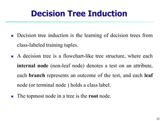
13
Decision Tree Induction
 Decision tree induction is the learning of decision trees from
class-labeled training tuples.
 A decision tree is a flowchart-like tree structure, where each
internal node (non-leaf node) denotes a test on an attribute,
each branch represents an outcome of the test, and each leaf
node (or terminal node ) holds a class label.
 The topmost node in a tree is the root node.

14
Decision Tree Induction: Training Dataset
age income student credit_rating buys_computer
<=30 high no fair no
<=30 high no excellent no
31…40 high no fair yes
>40 medium no fair yes
>40 low yes fair yes
>40 low yes excellent no
31…40 low yes excellent yes
<=30 medium no fair no
<=30 low yes fair yes
>40 medium yes fair yes
<=30 medium yes excellent yes
31…40 medium no excellent yes
31…40 high yes fair yes
>40 medium no excellent no

15
Output: A Decision Tree for “buys_computer”
age?
student? credit rating?
no yes yes
yes
31….40

16
How are decision trees used for
classification?
 Given a tuple, X, for which the associated class label is
unknown.
 The attribute values of the tuple are tested against the decision
tree.
 A path is traced from the root to a leaf node, which holds the
class prediction for that tuple.
 Decision trees can easily be converted to classification rules.

17
Why are decision tree classifiers so
popular?
 The construction of decision tree classifiers does not require any
domain knowledge or parameter setting, and therefore is
appropriate for exploratory knowledge discovery. Decision
trees can handle multidimensional data.
 Their representation of acquired knowledge in tree form is
intuitive and generally easy to understand by humans.
 The learning and classification steps of decision tree induction are
simple and fast. In general, decision tree classifiers have good
accuracy.

Attribute Selection Criteria
18
 It is used to determine the splitting criterion.

19
Attribute Selection Criteria
 A is discrete-valued: In this case, the outcomes of the test at
node N correspond directly to the known values of A.
 A is continuous-valued: In this case, the test at node N has two
possible outcomes, corresponding to the conditions A <= split
point and A >= split point, respectively.
 A is discrete-valued in Set form.

Information Gain
20
• Information gain is the basic criterion to decide whether a
feature should be used to split a node or not.
 Entropy: an information theory metric that measures the
impurity or uncertainty in a group of observations.
 It determines how a decision tree chooses to split data.

21
Attribute Selection Measure:
Information Gain
 Select the attribute with the highest information gain
 Let pi be the non- zero probability that an arbitrary tuple in D
belongs to class Ci, estimated by |Ci, D|/|D|
 Initial entropy:
A log function to the base 2 is used, because the information
is encoded in bits.
 New entropy (after using A to split D into v partitions) to
classify D:
 Information gained by branching on attribute A
)
(
log
)
( 2
1
i
m
i
i p
p
D
Info 



)
(
|
|
|
|
)
(
1
j
v
j
j
A D
Info
D
D
D
Info 
 

(D)
Info
Info(D)
Gain(A) A



28
Information Gain

29
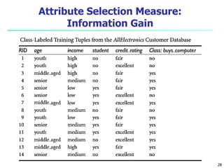
Information Gain
• The class label attribute, buys_computer, has two distinct
values (namely, {yes, no}); therefore, there are two distinct
classes (i.e., m = 2).
• There are nine tuples of class yes and five tuples of class
no.
)
(
log
)
( 2
1
i
m
i
i p
p
D
Info 




30
We need to look at the distribution of yes and no tuples for each
category of age. For the age category “youth,” there are two yes
tuples and three no tuples. For the category “middle aged,”
there are four yes tuples and zero no tuples. For the category
“senior,” there are three yes tuples and two no tuples.

32
Gain Ratio
Gain(Income) = 0.029
Gain Ratio (Income) = 0.029 / 1.557 = 0.019
A test on income splits the data into three partitions, namely low,
medium, and high, containing four, six, and four tuples,
respectively.

33
Gini Index
The Gini index is used in CART. Using the notation previously
described, the Gini index measures the impurity of D, a data
partition or set of training tuples, as

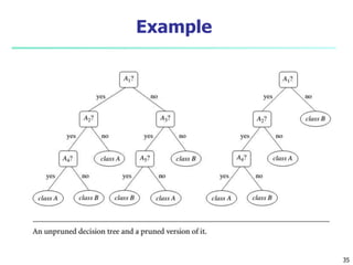
34
Over-fitting and Tree Pruning
 Over-fitting: An induced tree may over-fit the training data
 Too many branches, some may reflect anomalies due to noise or
outliers
 Two approaches to avoid over-fitting
 Pre-pruning: Halt tree construction early—do not split a node if
this would result in the goodness measure falling below a threshold
 Difficult to choose an appropriate threshold
 Post-pruning: Remove branches from a “fully grown” tree—get
a sequence of progressively pruned trees
 Use a set of data different from the training data to decide
which is the “best pruned tree”

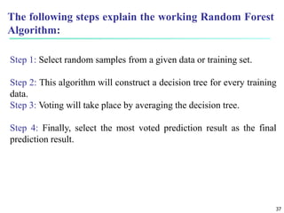
36
A Random Forest Algorithm is a supervised machine learning algorithm that
is extremely popular and is used for Classification and Regression problems in
Machine Learning.
We know that a forest comprises numerous trees, and the more trees more it
will be robust. Similarly, the greater the number of trees in a Random
Forest Algorithm, the higher its accuracy and problem-solving ability.
 Random Forest is a classifier that contains several decision trees on
various subsets of the given dataset and takes the average to improve the
predictive accuracy of that dataset.
 It is based on the concept of ensemble learning which is a process of
combining multiple classifiers to solve a complex problem and improve the
performance of the model.
Random Forest

37
Step 1: Select random samples from a given data or training set.
Step 2: This algorithm will construct a decision tree for every training
data.
Step 3: Voting will take place by averaging the decision tree.
Step 4: Finally, select the most voted prediction result as the final
prediction result.
The following steps explain the working Random Forest
Algorithm:

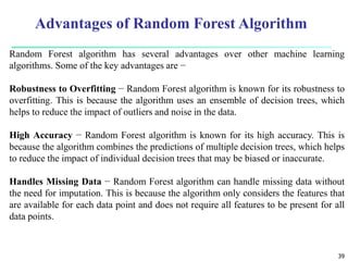
39
Random Forest algorithm has several advantages over other machine learning
algorithms. Some of the key advantages are −
Robustness to Overfitting − Random Forest algorithm is known for its robustness to
overfitting. This is because the algorithm uses an ensemble of decision trees, which
helps to reduce the impact of outliers and noise in the data.
High Accuracy − Random Forest algorithm is known for its high accuracy. This is
because the algorithm combines the predictions of multiple decision trees, which helps
to reduce the impact of individual decision trees that may be biased or inaccurate.
Handles Missing Data − Random Forest algorithm can handle missing data without
the need for imputation. This is because the algorithm only considers the features that
are available for each data point and does not require all features to be present for all
data points.
Advantages of Random Forest Algorithm

40
Non-Linear Relationships − Random Forest algorithm can handle non-linear
relationships between the features and the target variable. This is because the
algorithm uses decision trees, which can model non-linear relationships.
Feature Importance − Random Forest algorithm can provide information about
the importance of each feature in the model. This information can be used to
identify the most important features in the data and can be used for feature
selection and feature engineering.

42
Bayesian Classification: Why?
 It is a statistical classifier, it can predict class membership
probabilities such as the probability that a given tuple belongs to
a particular class.
 It is based on Bayes’ Theorem.
 A simple Bayesian classifier, naïve Bayesian classifier, has
comparable performance with decision tree and selected neural
network classifiers

43
Bayesian Theorem: Basics
 Let X be a data sample (“evidence”): class label is unknown.
 Let H be a hypothesis that X belongs to class C.
 Classification is to determine P(H|X) is the posteriori probability,
of H conditioned on X.
 X is a 35-year-old customer with an income of $40,000.
 Then P(H/X) reflects the probability that customer X will buy a
computer given that we know the customer’s age and income.
 In contrast, P(H) is the prior probability, of H .
 For our example, this is the probability that any given customer will
buy a computer, regardless of age, income, or any other
information.
 P(H), which is independent of X.

Bayesian Theorem: Basics
44
 P(X|H) (posteriori probability), the probability of X
conditioned on H. That is, it is the probability that a customer,
X, is 35 years old and earns $40,000, given that we know the
customer will buy a computer.
 P(X) is the prior probability of X.
 Using our example, it is the probability that a person from our
set of customers is 35 years old and earns $40,000.

45
Bayesian Theorem
 Given training data X, posteriori probability of a hypothesis H,
P(H|X), follows the Bayes theorem
)
(
)
(
)
|
(
)
|
(
X
X
X
P
H
P
H
P
H
P 

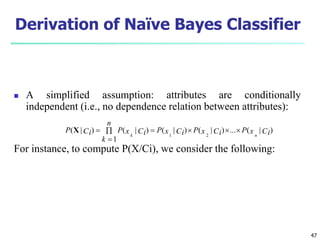
46
Derivation of Naïve Bayesian Classifier
 Let D be a training set of tuples and their associated class labels,
and each tuple is represented by an n-D attribute vector X = (x1,
x2, …, xn)
 Suppose there are m classes C1, C2, …, Cm.
 Classification is to derive the maximum posteriori, i.e., the
maximal P(Ci|X)
 This can be derived from Bayes’ theorem
 Since P(X) is constant for all classes, only
needs to be maximized
)
(
)
(
)
|
(
)
|
(
X
X
X
P
i
C
P
i
C
P
i
C
P 
)
(
)
|
(
)
|
(
i
C
P
i
C
P
i
C
P X
X 

47
Derivation of Naïve Bayes Classifier
 A simplified assumption: attributes are conditionally
independent (i.e., no dependence relation between attributes):
For instance, to compute P(X/Ci), we consider the following:
)
|
(
...
)
|
(
)
|
(
1
)
|
(
)
|
(
2
1
Ci
x
P
Ci
x
P
Ci
x
P
n
k
Ci
x
P
Ci
P
n
k







X

48
Naïve Bayesian Classifier: Training Dataset
Class:
C1:buys_computer = ‘yes’
C2:buys_computer = ‘no’
Data sample
X = (age <=30,
Income = medium,
Student = yes
Credit_rating = Fair)
age income student
credit_rating
buys_compu
<=30 high no fair no
<=30 high no excellent no
31…40 high no fair yes
>40 medium no fair yes
>40 low yes fair yes
>40 low yes excellent no
31…40 low yes excellent yes
<=30 medium no fair no
<=30 low yes fair yes
>40 medium yes fair yes
<=30 medium yes excellent yes
31…40 medium no excellent yes
31…40 high yes fair yes
>40 medium no excellent no

49
Naïve Bayesian Classifier: An Example
 P(Ci): P(buys_computer = “yes”) = 9/14 = 0.643
P(buys_computer = “no”) = 5/14= 0.357
 Compute P(X|Ci) for each class
P(age = “<=30” | buys_computer = “yes”) = 2/9 = 0.222
P(age = “<= 30” | buys_computer = “no”) = 3/5 = 0.6
P(income = “medium” | buys_computer = “yes”) = 4/9 = 0.444
P(income = “medium” | buys_computer = “no”) = 2/5 = 0.4
P(student = “yes” | buys_computer = “yes) = 6/9 = 0.667
P(student = “yes” | buys_computer = “no”) = 1/5 = 0.2
P(credit_rating = “fair” | buys_computer = “yes”) = 6/9 = 0.667
P(credit_rating = “fair” | buys_computer = “no”) = 2/5 = 0.4
 X = (age <= 30 , income = medium, student = yes, credit_rating = fair)
P(X|Ci) : P(X|buys_computer = “yes”) = 0.222 x 0.444 x 0.667 x 0.667 = 0.044
P(X|buys_computer = “no”) = 0.6 x 0.4 x 0.2 x 0.4 = 0.019
P(X|Ci)*P(Ci) : P(X|buys_computer = “yes”) * P(buys_computer = “yes”) = 0.028
P(X|buys_computer = “no”) * P(buys_computer = “no”) = 0.007
Therefore, X belongs to class (“buys_computer = yes”)

50
Naïve Bayesian Classifier: Comments
 Advantages
 Easy to implement
 Good results obtained in most of the cases
 Disadvantages
 Assumption: class conditional independence, therefore loss of
accuracy
 Practically, dependencies exist among variables
 E.g., hospitals: patients: Profile: age, family history, etc.
Symptoms: fever, cough etc., Disease: lung cancer, diabetes, etc.
 Dependencies among these cannot be modeled by Naïve Bayesian
Classifier

Types of Naive Bayes Classifier
 Multinominal, Gaussian and Bernoulli Naive Bayes
are the three types of Naïve Bayes classification:
Multinomial Naive Bayes:
 This is mostly used for document classification
problem, i.e whether a document belongs to the
category of sports, politics, technology etc. The
features/predictors used by the classifier are the
frequency of the words present in the document.
51

Bernoulli Naive Bayes:
 This is similar to the multinomial naive bayes but
the predictors are boolean variables. The
parameters that we use to predict the class
variable take up only values yes or no, for
example if a word occurs in the text or not.
52

Gaussian Naive Bayes:
 When the predictors take up a continuous value
and are not discrete, we assume that these values
are sampled from a Gaussian distribution.
 Since the way, the values are present in the
dataset changes, the formula for conditional
probability changes to,
53

Conclusion
Naive Bayes algorithms are mostly used in
sentiment analysis,
spam filtering,
recommendation systems
They are fast and easy to implement but their
biggest disadvantage is that the requirement of
predictors to be independent.
In most of the real life cases, the predictors are
dependent, this hinders the performance of the
classifier.
54

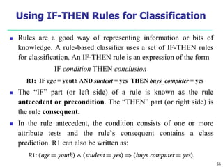
56
Using IF-THEN Rules for Classification
 Rules are a good way of representing information or bits of
knowledge. A rule-based classifier uses a set of IF-THEN rules
for classification. An IF-THEN rule is an expression of the form
IF condition THEN conclusion
R1: IF age = youth AND student = yes THEN buys_computer = yes
 The “IF” part (or left side) of a rule is known as the rule
antecedent or precondition. The “THEN” part (or right side) is
the rule consequent.
 In the rule antecedent, the condition consists of one or more
attribute tests and the rule’s consequent contains a class
prediction. R1 can also be written as:

57
Using IF-THEN Rules for Classification
 If the condition holds true for a given tuple, we say that the rule
antecedent is satisfied and that rule covers the tuple.
 Assessment of a rule: coverage and accuracy
 ncovers = # of tuples covered by R
 ncorrect = # of tuples correctly classified by R
coverage(R) = ncovers / |D| /* D: training data set */
accuracy(R) = ncorrect / ncovers

58
age?
student? credit rating?
<=30 >40
no yes yes
yes
31..40
fair
excellent
yes
no
 Example: Rule extraction from our buys_computer decision-tree
IF age = young AND student = no THEN buys_computer = no
IF age = young AND student = yes THEN buys_computer = yes
IF age = mid-age THEN buys_computer = yes
IF age = old AND credit_rating = excellent THEN buys_computer = no
IF age = young AND credit_rating = fair THEN buys_computer = yes
Rule Extraction from a Decision Tree
 Rules are easier to understand than large trees
 One rule is created for each path from the root to a
leaf
 Each attribute-value pair along a path forms a
conjunction: the leaf holds the class prediction
 Rules are mutually exclusive and exhaustive

60
Classification by Backpropagation
 Back propagation: A neural network learning algorithm
Started by psychologists and neurobiologists to develop and
test computational analogues of neurons
 A neural network: A set of connected input/output units
where each connection has a weight associated with it
 During the learning phase, the network learns by adjusting
the weights so as to be able to predict the correct class label of
the input tuples
 Also referred to as connectionist learning due to the
connections between units

61
Neural Network as a Classifier
 Weakness
 Long training time
 Require a number of parameters typically best determined empirically,
e.g., the network topology or ``structure."
 Strength
 High tolerance to noisy data
 Ability to classify untrained patterns
 Well-suited for continuous-valued inputs and outputs
 Successful on a wide array of real-world data
 Algorithms are inherently parallel
 Techniques have recently been developed for the extraction of rules from
trained neural networks

62
A Neuron (= a perceptron)
 The n-dimensional input vector x is mapped into variable y by
means of the scalar product and a nonlinear function mapping
mk
-
f
weighted
sum
Input
vector x
output y
Activation
function
weight
vector w

w0
w1
wn
x0
x1
xn
)
sign(
y
Example
For
n
0
i
k
i
i x
w m

 


A Multi-Layer Feed-Forward Neural Network

64
How A Multi-Layer Neural Network Works?
 The inputs to the network correspond to the attributes measured
for each training tuple
 Inputs are fed simultaneously into the units making up the input
layer
 They are then weighted and fed simultaneously to a hidden layer
 The number of hidden layers is arbitrary, although usually only one
 The weighted outputs of the last hidden layer are input to units
making up the output layer, which emits the network's prediction
 The network is feed-forward in that none of the weights cycles
back to an input unit or to an output unit of a previous layer
 From a statistical point of view, networks perform nonlinear
regression: Given enough hidden units and enough training
samples, they can closely approximate any function

65
Defining a Network Topology
 First decide the network topology: # of units in the input layer,
# of hidden layers (if > 1), # of units in each hidden layer, and #
of units in the output layer
 Normalizing the input values for each attribute measured in the
training tuples to [0.0—1.0]
 One input unit per domain value, each initialized to 0
 Output, if for classification and more than two classes, one
output unit per class is used
 Once a network has been trained and its accuracy is
unacceptable, repeat the training process with a different
network topology or a different set of initial weights

66
Backpropagation
 Iteratively process a set of training tuples & compare the network's
prediction with the actual known target value
 For each training tuple, the weights are modified to minimize the mean
squared error between the network's prediction and the actual target
value
 Modifications are made in the “backwards” direction: from the output
layer, through each hidden layer down to the first hidden layer, hence
“backpropagation”
 Steps
 Initialize weights (to small random #s) and biases in the network
 Propagate the inputs forward (by applying activation function)
 Backpropagate the error (by updating weights and biases)
 Terminating condition (when error is very small, etc.)

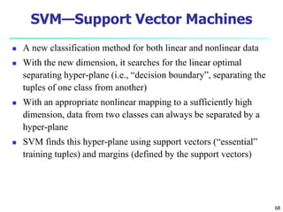
68
SVM—Support Vector Machines
 A new classification method for both linear and nonlinear data
 With the new dimension, it searches for the linear optimal
separating hyper-plane (i.e., “decision boundary”, separating the
tuples of one class from another)
 With an appropriate nonlinear mapping to a sufficiently high
dimension, data from two classes can always be separated by a
hyper-plane
 SVM finds this hyper-plane using support vectors (“essential”
training tuples) and margins (defined by the support vectors)

69
SVM—History and Applications
 Vapnik and colleagues (1992)—groundwork from Vapnik
& Chervonenkis’ statistical learning theory in 1960s
 Features: training can be slow but accuracy is high owing
to their ability to model complex nonlinear decision
boundaries (margin maximization)
 Used both for classification and prediction
 Applications:
 handwritten digit recognition, object recognition,
speaker identification, benchmarking time-series
prediction tests

70
SVM—General Philosophy
Support Vectors
Small Margin Large Margin

71
SVM—Margins and Support Vectors

72
SVM—When Data Is Linearly Separable
m
Let data D be (X1, y1), …, (X|D|, y|D|), where Xi is the set of training tuples
associated with the class labels yi
There are infinite lines (hyperplanes) separating the two classes but we want to
find the best one (the one that minimizes classification error on unseen data)
SVM searches for the hyperplane with the largest margin, i.e., maximum
marginal hyperplane (MMH)

73
SVM—Linearly Separable
 A separating hyperplane can be written as
W . X + b = 0
where W={w1, w2, …, wn} is a weight vector and b a scalar (bias)
 For 2-D it can be written as
w0 + w1 x1 + w2 x2 = 0
 The hyperplane defining the sides of the margin:
H1: w0 + w1 x1 + w2 x2 ≥ 1 for yi = +1, and
H2: w0 + w1 x1 + w2 x2 ≤ – 1 for yi = –1
 Any training tuples that fall on hyperplanes H1 or H2 (i.e., the
sides defining the margin) are support vectors
 This becomes a constrained (convex) quadratic optimization problem:
Quadratic objective function and linear constraints  Quadratic
Programming (QP)  Lagrangian multipliers

74
SVM—Linearly Inseparable
 Transform the original input data into a higher dimensional
space
 Search for a linear separating hyperplane in the new space
A1
A2

75
SVM vs. Neural Network
 SVM
 Relatively new concept
 Deterministic algorithm
 Nice Generalization
properties
 Hard to learn – learned in
batch mode using
quadratic programming
techniques
 Using kernels can learn
very complex functions
 Neural Network
 Relatively old
 Nondeterministic algorithm
 Generalizes well but
doesn’t have strong
mathematical foundation
 Can easily be learned in
incremental fashion
 To learn complex
functions—use multilayer
perceptron (not that trivial)

classification in data warehouse and mining

More Related Content

classification in data warehouse and mining