Cluster analysis

Data Analysis Course
Cluster Analysis and Decision
Trees(version-1)
Venkat Reddy

• Data analysis design document
• Introduction to statistical data analysis
• Descriptive statistics
• Data exploration, validation & sanitization
• Probability distributions examples and applications

Venkat Reddy
• Simple correlation and regression analysis
• Multiple liner regression analysis
• Logistic regression analysis
• Testing of hypothesis

• Clustering and Decision trees
• Time series analysis and forecasting
• Credit Risk Model building-1 2
• Credit Risk Model building-2

Note
• This presentation is just class notes. The course notes for Data
Analysis Training is by written by me, as an aid for myself.
• The best way to treat this is as a high-level summary; the
actual session went more in depth and contained other

Venkat Reddy
information.
• Most of this material was written as informal notes, not
intended for publication
• Please send questions/comments/corrections to
venkat@trenwiseanalytics.com or 21.venkat@gmail.com
• Please check my website for latest version of this document
-Venkat Reddy 3

Contents
• What is the need of Segmentation
• Introduction to Segmentation & Cluster analysis
• Applications of Cluster Analysis
• Types of Clusters

Venkat Reddy
• Building Partitional Clusters
• K means Clustering & Analysis
• Building Decision Trees
• CHAID Segmentation & Analysis

4

What is the need of segmentation?
Problem:
• 10,000 Customers - we know their age, city name, income,
employment status, designation
• You have to sell 100 Blackberry phones(each costs $1000) to

Venkat Reddy
the people in this group. You have maximum of 7 days
• If you start giving demos to each individual, 10,000 demos will
take more than one year. How will you sell maximum number
of phones by giving minimum number of demos?

5

What is the need of segmentation?
Solution
• Divide the whole population into two groups employed / unemployed
• Further divide the employed population into two groups high/low salary
• Further divide that group into high /low designation

10000
customers

Venkat Reddy
Unemployed Employed
3000 7000

Low salary High Salary
5000 2000

Low High
6
Designation Designation
1800 200

Segmentation and Cluster Analysis
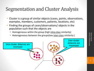
• Cluster is a group of similar objects (cases, points, observations,
examples, members, customers, patients, locations, etc)
• Finding the groups of cases/observations/ objects in the
population such that the objects are
• Homogeneous within the group (high intra-class similarity)

Venkat Reddy
• Heterogeneous between the groups(low inter-class similarity )

Inter-cluster
distances are
Intra-cluster distances are
maximized
minimized

7

Applications of Cluster Analysis
• Market Segmentation: Grouping people (with the willingness,
purchasing power, and the authority to buy) according to their
similarity in several dimensions related to a product under
consideration.
• Sales Segmentation: Clustering can tell you what types of customers
buy what products

Venkat Reddy
• Credit Risk: Segmentation of customers based on their credit history
• Operations: High performer segmentation & promotions based on
person’s performance
• Insurance: Identifying groups of motor insurance policy holders with
a high average claim cost.
• City-planning: Identifying groups of houses according to their house
type, value, and geographical location
• Geographical: Identification of areas of similar land use in an earth
8
observation database.

Types of Clusters
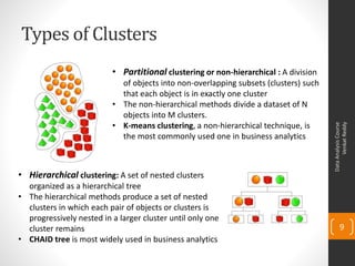
• Partitional clustering or non-hierarchical : A division
of objects into non-overlapping subsets (clusters) such
that each object is in exactly one cluster
• The non-hierarchical methods divide a dataset of N
objects into M clusters.
• K-means clustering, a non-hierarchical technique, is

Venkat Reddy
the most commonly used one in business analytics

• Hierarchical clustering: A set of nested clusters
organized as a hierarchical tree
• The hierarchical methods produce a set of nested
clusters in which each pair of objects or clusters is
progressively nested in a larger cluster until only one
cluster remains 9
• CHAID tree is most widely used in business analytics

Cluster Analysis -Example
Maths Science Gk Apt Maths Science Gk Apt
Student-1 94 82 87 89 Student-1 94 82 87 89
Student-2 46 67 33 72 Student-2 46 67 33 72
Student-3 98 97 93 100 Student-3 98 97 93 100
Student-4 14 5 7 24 Student-4 14 5 7 24
Student-5 86 97 95 95 Student-5 86 97 95 95
Student-6 34 32 75 66 Student-6 34 32 75 66
Student-7 69 44 59 55 Student-7 69 44 59 55

Venkat Reddy
Student-8 85 90 96 89 Student-8 85 90 96 89
Student-9 24 26 15 22 Student-9 24 26 15 22

Maths Science Gk Apt
Student-4 14 5 7 24
2,7
Student-9 24 26 15 22
4,9,6
Student-6 34 32 75 66
Student-2 46 67 33 72
Student-7 69 44 59 55 8,5,1,3
Student-8 85 90 96 89
Student-5 86 97 95 95 10
Student-1 94 82 87 89
Student-3 98 97 93 100

Building Clusters
1. Select a distance measure
2. Select a clustering algorithm
3. Define the distance between two clusters
4. Determine the number of clusters
5. Validate the analysis

Venkat Reddy
• The aim is to build clusters i.e divide the whole population into group of similar
objects
• What is similarity/dis-similarity? 11
• How do you define distance between two clusters

Distance measures
• To measure similarity between two observations a
distance measure is needed. With a single variable,
similarity is straightforward
• Example: income – two individuals are similar if their income
level is similar and the level of dissimilarity increases as the

Venkat Reddy
income gap increases
• Multiple variables require an aggregate distance
measure
• Many characteristics (e.g. income, age, consumption habits,
family composition, owning a car, education level, job…), it
becomes more difficult to define similarity with a single value
• The most known measure of distance is the Euclidean
distance, which is the concept we use in everyday life for 12
spatial coordinates.

Examples of distances
A
 x  xkj 
n
2
Dij  ki
Euclidean distance
k 1 B
n A
Dij   xki  xkj City-block (Manhattan) distance
k 1 B

Venkat Reddy
Dij distance between cases i and j xkj - value of variable xk for case j

Other distance measures: Chebychev, Minkowski, Mahalanobis,
maximum distance, cosine similarity, simple correlation between
observations etc.,
Data matrix Dissimilarity matrix
 x11 ... x1f ... x1p   0 
   d(2,1) 
 ... ... ... ... ... 
 0  13
x ... xif ... xip   d(3,1) d ( 3,2) 0 
 i1   
 ... ... ... ... ...   : : : 
x xnp  d ( n,1) d ( n,2) ...
 ... xnf ...   ... 0

 n1 

K -Means Clustering – Algorithm
1. The number k of clusters is fixed
2. An initial set of k “seeds” (aggregation centres) is provided
1. First k elements
2. Other seeds (randomly selected or explicitly defined)
3. Given a certain fixed threshold, all units are assigned to the

Venkat Reddy
nearest cluster seed
4. New seeds are computed
5. Go back to step 3 until no reclassification is necessary

Or simply
Initialize k cluster centers
Do
Assignment step: Assign each data point to its closest cluster center
Re-estimation step: Re-compute cluster centers 14
While (there are still changes in the cluster centers)

K Means clustering in action
• Dividing the data into 10 clusters using K-Means

Distance metric will
decide cluster for
these points

Venkat Reddy
15

SAS Code & Options
proc fastclus data= mylib.super_market_data
radius=0 replace=full maxclusters =3 maxiter =20 list distance;
id cust_id;
var age income spend family_size visit_Other_shops;
run;

Options

Venkat Reddy
• The RADIUS= option establishes the minimum distance criterion for selecting new
seeds. No observation is considered as a new seed unless its minimum distance to
previous seeds exceeds the value given by the RADIUS= option. The default value is 0.
• The MAXCLUSTERS= option specifies the maximum number of clusters allowed. If you
omit the MAXCLUSTERS= option, a value of 100 is assumed.
• The REPLACE= option specifies how seed replacement is performed.
• FULL :requests default seed replacement.
• PART :requests seed replacement only when the distance between the observation and the
closest seed is greater than the minimum distance between seeds.
• NONE : suppresses seed replacement.
16
• RANDOM :Selects a simple pseudo-random sample of complete observations as initial cluster
seeds.

SAS Code & Options
• The MAXITER= option specifies the maximum number of iterations for re
computing cluster seeds. When the value of the MAXITER= option is greater
than 0, each observation is assigned to the nearest seed, and the seeds are
recomputed as the means of the clusters.
• The LIST option lists all observations, giving the value of the ID variable (if
any), the number of the cluster to which the observation is assigned, and

Venkat Reddy
the distance between the observation and the final cluster seed.
• The DISTANCE option computes distances between the cluster means.
• The ID variable, which can be character or numeric, identifies observations
on the output when you specify the LIST option.
• The VAR statement lists the numeric variables to be used in the cluster
analysis. If you omit the VAR statement, all numeric variables not listed in
other statements are used.

17

Lab- Clustering
• Retail Analytics problem: Supermarket data. A super market want to
give a special discount to few selected customers. The aim to
increase the sales by studying the buying capacity of the customers
• Find the customer segments using cluster analysis code(do not
mention maxclusters)

Venkat Reddy
• How many clusters have been created?
• What are the properties of customers in each cluster?
• Analyze the output and identify the customer group with good
income, high spend, large family size.
• How much time does it take to create the clusters?
• Now create 5 clusters using K means clustering techniques
• Find the target customer group
• Further clustering in cluster 3? 18

SAS output interpretation
• RMSSTD - Pooled standard deviation of all the variables forming the cluster.
Since the objective of cluster analysis is to form homogeneous groups, the
• RMSSTD of a cluster should be as small as possible
• SPRSQ -Semipartial R-squared is a measure of the homogeneity of merged
clusters, so SPRSQ is the loss of homogeneity due to combining two groups
or clusters to form a new group or cluster.

Venkat Reddy
• Thus, the SPRSQ value should be small to imply that we are merging two
homogeneous groups
• RSQ (R-squared) measures the extent to which groups or clusters are
different from each other
• So, when you have just one cluster RSQ value is, intuitively, zero). Thus, the RSQ
value should be high.
• Centroid Distance is simply the Euclidian distance between the centroid of
the two clusters that are to be joined or merged.
• So, Centroid Distance is a measure of the homogeneity of merged clusters and the 19
value should be small.

Hierarchical Clustering -Decision
Trees
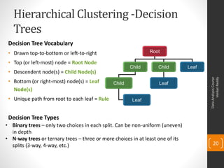
Decision Tree Vocabulary
• Drawn top-to-bottom or left-to-right Root

• Top (or left-most) node = Root Node
Child Child Leaf
• Descendent node(s) = Child Node(s)

Venkat Reddy
• Bottom (or right-most) node(s) = Leaf Child Leaf
Node(s)
• Unique path from root to each leaf = Rule Leaf

Decision Tree Types
• Binary trees – only two choices in each split. Can be non-uniform (uneven)
in depth
• N-way trees or ternary trees – three or more choices in at least one of its
splits (3-way, 4-way, etc.) 20

Decision Tree-Example
Maths Science Gk Apt Maths Science Gk Apt
Student-1 94 82 87 89 Student-1 94 82 87 89
Student-2 46 67 33 72 Student-2 46 67 33 72
Student-3 98 97 93 100 Student-3 98 97 93 100
Student-4 14 5 7 24 Student-4 14 5 7 24
Student-5 86 97 95 95 Student-5 86 97 95 95
Student-6 34 32 75 66 Student-6 34 32 75 66
Student-7 69 44 59 55 Student-7 69 44 59 55

Venkat Reddy
Student-8 85 90 96 89 Student-8 85 90 96 89
Student-9 24 26 15 22 Student-9 24 26 15 22

Maths Science Gk Apt
Student-4 14 5 7 24 1-10
Student-9 24 26 15 22
Student-6 34 32 75 66
2,7,8,5,1,
Student-2 46 67 33 72 4,9,6
3
Student-7 69 44 59 55
Student-8 85 90 96 89
Student-5 86 97 95 95 2,7 8,5,1,3 21
Student-1 94 82 87 89
Student-3 98 97 93 100

Decision Trees Algorithm

(1) Which attribute to start?

Venkat Reddy
(2) Which node to proceed?

(3) Which attribute to proceed with?

(4) When to stop/ come to conclusion?

1. Start with best split attribute at root 22
2. Split the population into heterogeneous groups
3. Go to each group and repeat step 1 and 2 until there is no further best split

Best Splitting attribute
• The best split at root(or child) nodes is defined as one that does the
best job of separating the data into groups where a single class
predominates in each group
• Example: Population data input variables/attributes include: Height,
Gender, Age

Venkat Reddy
• Split the above according to the above “best split” rule
• Measure used to evaluate a potential split is purity
• The best split is one that increases purity of the sub-sets by the greatest
amount
• Purity (Diversity) Measures:
• Gini (population diversity)
• Entropy (information gain)
• Information Gain Ratio
• Chi-square Test 23

Clustering SAS Code & Options
proc cluster data= mylib.cluster_data
simple noeigen method=centroid rmsstd rsquare nonorm out=tree;
id cust_id;
var age income spend family_size Other_shops;
run;
Options

Venkat Reddy
• SIMPLE: The simple option displays simple, descriptive statistics.
• NOEIGEN: The noeigen option suppresses computation of eigenvalues. Specifying
the noeigen option saves time if the number of variables is large
• The METHOD= specification determines the clustering method used by the
procedure. Here, we are using CENTROID method.
• The RMSSTD option displays the root-mean-square standard deviation of each cluster.
• The RSQUARE option displays the R2 and semipartial R2 to evaluate cluster solution.
• The NONORM option prevents the distances from being normalized to unit mean or
unit root mean square with most methods.
24

Lab: Hierarchical clustering
• Build hierarchical clusters for the supermarket data
• Draw the tree diagram
• What are the properties of customers in each cluster?
• Analyze the output and identify the customer group with good

Venkat Reddy
income, high spend, large family size.

25

SAS output interpretation
• RMSSTD - Pooled standard deviation of all the variables forming the cluster.
Since the objective of cluster analysis is to form homogeneous groups, the
• RMSSTD of a cluster should be as small as possible
• SPRSQ -Semipartial R-squared is a measure of the homogeneity of merged
clusters, so SPRSQ is the loss of homogeneity due to combining two groups
or clusters to form a new group or cluster.

Venkat Reddy
• Thus, the SPRSQ value should be small to imply that we are merging two
homogeneous groups
• RSQ (R-squared) measures the extent to which groups or clusters are
different from each other
• So, when you have just one cluster RSQ value is, intuitively, zero). Thus, the RSQ
value should be high.
• Centroid Distance is simply the Euclidian distance between the centroid of
the two clusters that are to be joined or merged.
• So, Centroid Distance is a measure of the homogeneity of merged clusters and the 26
value should be small.

CHAID Segmentation
• CHAID- Chi-Squared Automatic Interaction Detector
• CHAID is a non-binary decision tree.
• The decision or split made at each node is still based on a single
variable, but can result in multiple branches.
• The split search algorithm is designed for categorical variables.

Venkat Reddy
• Continuous variables must be grouped into a finite number of bins
to create categories.
• A reasonable number of “equal population bins” can be created for
use with CHAID.
• ex. If there are 1000 samples, creating 10 equal population bins
would result in 10 bins, each containing 100 samples.

• A Chi-square value is computed for each variable and used to
determine the best variable to split on. 27

CHAID Algorithm
1. Select significant independent variable
2. Identify category groupings or interval breaks to create
groups most different with respect to the dependent
variable

Venkat Reddy
3. Select as the primary independent variable the one
identifying groups with the most different values of the
dependent variable based on chi-square
4. Select additional variables to extend each branch if there are
further significant differences

28

Venkat Reddy Konasani
Manager at Trendwise Analytics
venkat@TrendwiseAnalytics.com
21.venkat@gmail.com

Venkat Reddy
+91 9886 768879

29

Cluster analysis

More Related Content

Cluster analysis