Location via proxy:   [ UP ]  
[Report a bug]   [Manage cookies]                
SlideShare a Scribd company logo
Chapter
McGraw-Hill/Irwin Copyright © 2009 by The McGraw-Hill Companies, Inc. All rights reserved.
6 Common Stock
Valuation
6-2
Learning Objectives
Separate yourself from the commoners by having a good
Understanding of these security valuation methods:
1. The basic dividend discount model.
2. The two-stage dividend growth model.
3. The residual income model.
4. Price ratio analysis.
6-3
Common Stock Valuation
• Our goal in this chapter is to examine the methods
commonly used by financial analysts to assess the
economic value of common stocks.
• These methods are grouped into three categories:
– Dividend discount models
– Residual Income models
– Price ratio models
6-4
Security Analysis: Be Careful Out There
• Fundamental analysis is a term for studying a
company’s accounting statements and other financial and
economic information to estimate the economic value of
a company’s stock.
• The basic idea is to identify “undervalued” stocks to buy
and “overvalued” stocks to sell.
• In practice however, such stocks may in fact be correctly
priced for reasons not immediately apparent to the
analyst.
6-5
The Dividend Discount Model
• The Dividend Discount Model (DDM) is a method to estimate the
value of a share of stock by discounting all expected future dividend
payments. The basic DDM equation is:
• In the DDM equation:
– P0 = the present value of all future dividends
– Dt = the dividend to be paid t years from now
– k = the appropriate risk-adjusted discount rate
       T
T
3
3
2
2
1
0
k
1
D
k
1
D
k
1
D
k
1
D
P







 
6-6
Example: The Dividend Discount Model
• Suppose that a stock will pay three annual dividends of
$200 per year, and the appropriate risk-adjusted discount
rate, k, is 8%.
• In this case, what is the value of the stock today?
     
     
$515.42
0.08
1
$200
0.08
1
$200
0.08
1
$200
P
k
1
D
k
1
D
k
1
D
P
3
2
0
3
3
2
2
1
0













6-7
The Dividend Discount Model:
the Constant Growth Rate Model
• Assume that the dividends will grow at a constant growth rate g. The
dividend next period (t + 1) is:
• For constant dividend growth for “T” years, the DDM formula
becomes:
g
k
if
D
T
P
g
k
if
k
1
g
1
1
g
k
g)
(1
D
P
0
0
T
1
0
























 
g)
(1
g)
(1
D
g)
(1
D
D
So,
g
1
D
D
0
1
2
t
1
t












6-8
Example: The Constant Growth Rate Model
• Suppose the current dividend is $10, the dividend growth rate is
10%, there will be 20 yearly dividends, and the appropriate discount
rate is 8%.
• What is the value of the stock, based on the constant growth rate
model?
  $243.86
1.08
1.10
1
.10
.08
1.10
$10
P
k
1
g
1
1
g
k
g)
(1
D
P
20
0
T
0
0







































6-9
The Dividend Discount Model:
the Constant Perpetual Growth Model.
• Assuming that the dividends will grow forever at a
constant growth rate g.
• For constant perpetual dividend growth, the DDM formula
becomes:
 
k)
g
:
(Important
g
k
D
g
k
g
1
D
P 1
0
0 






6-10
Example: Constant Perpetual Growth Model
• Think about the electric utility industry.
• In 2007, the dividend paid by the utility company, DTE Energy Co.
(DTE), was $2.12.
• Using D0 =$2.12, k = 6.7%, and g = 2%, calculate an estimated value
for DTE.
Note: the actual mid-2007 stock price of DTE was $47.81.
What are the possible explanations for the difference?
  $46.01
.02
.067
1.02
$2.12
P0 



6-11
The Dividend Discount Model:
Estimating the Growth Rate
• The growth rate in dividends (g) can be estimated in a
number of ways:
– Using the company’s historical average growth rate.
– Using an industry median or average growth rate.
– Using the sustainable growth rate.
6-12
The Historical Average Growth Rate
• Suppose the Broadway Joe Company paid the following dividends:
– 2002: $1.50 2005: $1.80
– 2003: $1.70 2006: $2.00
– 2004: $1.75 2007: $2.20
• The spreadsheet below shows how to estimate historical average
growth rates, using arithmetic and geometric averages.
Year: Dividend: Pct. Chg:
2007 $2.20 10.00%
2006 $2.00 11.11%
2005 $1.80 2.86% Grown at
2004 $1.75 2.94% Year: 7.96%:
2003 $1.70 13.33% 2002 $1.50
2002 $1.50 2003 $1.62
2004 $1.75
8.05% 2005 $1.89
2006 $2.04
7.96% 2007 $2.20
Arithmetic Average:
Geometric Average:
6-13
The Sustainable Growth Rate
• Return on Equity (ROE) = Net Income / Equity
• Payout Ratio = Proportion of earnings paid out as dividends
• Retention Ratio = Proportion of earnings retained for investment
Ratio)
Payout
-
(1
ROE
Ratio
Retention
ROE
Rate
Growth
e
Sustainabl




6-14
Example: Calculating and Using the
Sustainable Growth Rate
• In 2007, American Electric Power (AEP) had an ROE of 10.17%,
projected earnings per share of $2.25, and a per-share dividend of
$1.56. What was AEP’s:
– Retention rate?
– Sustainable growth rate?
• Payout ratio = $1.56 / $2.25 = .693
• So, retention ratio = 1 – .693 = .307 or 30.7%
• Therefore, AEP’s sustainable growth rate = .1017  .307 = .03122, or
3.122%
6-15
Example: Calculating and Using the
Sustainable Growth Rate, Cont.
• What is the value of AEP stock, using the perpetual growth model,
and a discount rate of 6.7%?
• The actual mid-2007 stock price of AEP was $45.41.
• In this case, using the sustainable growth rate to value the stock
gives a reasonably accurate estimate.
• What can we say about g and k in this example?
  $44.96
.03122
.067
1.03122
$1.56
P 



0
6-16
The Two-Stage Dividend Growth Model
• The two-stage dividend growth model assumes that a
firm will initially grow at a rate g1 for T years, and
thereafter grow at a rate g2 < k during a perpetual second
stage of growth.
• The Two-Stage Dividend Growth Model formula is:
2
2
0
T
1
T
1
1
1
0
g
k
)
g
(1
D
k
1
g
1
k
1
g
1
1
g
k
)
g
(1
D
P































0
6-17
Using the Two-Stage
Dividend Growth Model, I.
• Although the formula looks complicated, think of it as two
parts:
– Part 1 is the present value of the first T dividends (it is the same
formula we used for the constant growth model).
– Part 2 is the present value of all subsequent dividends.
• So, suppose MissMolly.com has a current dividend of
D0 = $5, which is expected to shrink at the rate, g1 = 10%
for 5 years, but grow at the rate, g2 = 4% forever.
• With a discount rate of k = 10%, what is the present value
of the stock?
6-18
Using the Two-Stage
Dividend Growth Model, II.
• The total value of $46.03 is the sum of a $14.25 present value of the
first five dividends, plus a $31.78 present value of all subsequent
dividends.
$46.03.
$31.78
$14.25
0.04
0.10
0.04)
$5.00(1
0.10
1
0.90
0.10
1
0.90
1
0.10)
(
0.10
)
$5.00(0.90
P
g
k
)
g
(1
D
k
1
g
1
k
1
g
1
1
g
k
)
g
(1
D
P
5
5
2
2
0
T
1
T
1
1
1
0































































0
0
6-19
Example: Using the DDM to Value a Firm
Experiencing “Supernormal” Growth, I.
• Chain Reaction, Inc., has been growing at a phenomenal rate of 30%
per year.
• You believe that this rate will last for only three more years.
• Then, you think the rate will drop to 10% per year.
• Total dividends just paid were $5 million.
• The required rate of return is 20%.
• What is the total value of Chain Reaction, Inc.?
6-20
Example: Using the DDM to Value a Firm
Experiencing “Supernormal” Growth, II.
• First, calculate the total dividends over the “supernormal” growth
period:
• Using the long run growth rate, g, the value of all the shares at Time
3 can be calculated as:
P3 = [D3 x (1 + g)] / (k – g)
P3 = [$10.985 x 1.10] / (0.20 – 0.10) = $120.835
Year Total Dividend: (in $millions)
1 $5.00 x 1.30 = $6.50
2 $6.50 x 1.30 = $8.45
3 $8.45 x 1.30 = $10.985
6-21
Example: Using the DDM to Value a Firm
Experiencing “Supernormal” Growth, III.
• Therefore, to determine the present value of the firm today, we need
the present value of $120.835 and the present value of the dividends
paid in the first 3 years:
       
       
million.
$87.58
$69.93
$6.36
$5.87
$5.42
0.20
1
$120.835
0.20
1
$10.985
0.20
1
$8.45
0.20
1
$6.50
P
k
1
P
k
1
D
k
1
D
k
1
D
P
3
3
2
3
3
3
3
2
2
1





















0
0
6-22
Discount Rates for
Dividend Discount Models
• The discount rate for a stock can be estimated using the capital
asset pricing model (CAPM ).
• We will discuss the CAPM in a later chapter.
• However, we can estimate the discount rate for a stock using this
formula:
Discount rate = time value of money + risk premium
= U.S. T-bill Rate + (Stock Beta x Stock Market Risk Premium)
T-bill Rate: return on 90-day U.S. T-bills
Stock Beta: risk relative to an average stock
Stock Market Risk Premium: risk premium for an average stock
6-23
Observations on Dividend
Discount Models, I.
Constant Perpetual Growth Model:
• Simple to compute
• Not usable for firms that do not pay dividends
• Not usable when g > k
• Is sensitive to the choice of g and k
• k and g may be difficult to estimate accurately.
• Constant perpetual growth is often an unrealistic assumption.
6-24
Observations on Dividend
Discount Models, II.
Two-Stage Dividend Growth Model:
• More realistic in that it accounts for two stages of growth
• Usable when g > k in the first stage
• Not usable for firms that do not pay dividends
• Is sensitive to the choice of g and k
• k and g may be difficult to estimate accurately.
6-25
Residual Income Model (RIM), I.
• We have valued only companies that pay dividends.
– But, there are many companies that do not pay dividends.
– What about them?
– It turns out that there is an elegant way to value these
companies, too.
• The model is called the Residual Income Model (RIM).
• Major Assumption (known as the Clean Surplus Relationship, or
CSR): The change in book value per share is equal to earnings per
share minus dividends.
6-26
Residual Income Model (RIM), II.
• Inputs needed:
– Earnings per share at time 0, EPS0
– Book value per share at time 0, B0
– Earnings growth rate, g
– Discount rate, k
• There are two equivalent formulas for the Residual Income Model:
g
k
g
B
EPS
P
or
g
k
k
B
g)
(1
EPS
B
P
0
1
0
0
0
0
0










BTW, it turns out that the
RIM is mathematically the
same as the constant
perpetual growth model.
6-27
Using the Residual Income Model.
• Superior Offshore International, Inc. (DEEP)
• It is July 1, 2007—shares are selling in the market for $10.94.
• Using the RIM:
– EPS0 = $1.20
– DIV = 0
– B0 = $5.886
– g = 0.09
– k = .13
• What can we say
about the market
price of DEEP? $19.46.
.04
$.7652
$1.308
$5.886
P
.09
.13
.13
$5.886
.09)
(1
$1.20
$5.886
P
g
k
k
B
g)
(1
EPS
B
P
0
0
0
0
0
0


















6-28
DEEP Growth
• Using the information from the previous slide, what growth rate
results in a DEEP price of $10.94?
3.55%.
or
.0355
g
6.254g
.2222
.4348
1.20g
5.054g
$.6570
.7652
1.20g
1.20
g)
(.13
$5.054
g
.13
.13
$5.886
g)
(1
$1.20
$5.886
$10.94
g
k
k
B
g)
(1
EPS
B
P 0
0
0
0
























6-29
Price Ratio Analysis, I.
• Price-earnings ratio (P/E ratio)
– Current stock price divided by annual earnings per share (EPS)
• Earnings yield
– Inverse of the P/E ratio: earnings divided by price (E/P)
• High-P/E stocks are often referred to as growth stocks,
while low-P/E stocks are often referred to as value
stocks.
6-30
Price Ratio Analysis, II.
• Price-cash flow ratio (P/CF ratio)
– Current stock price divided by current cash flow per share
– In this context, cash flow is usually taken to be net income plus
depreciation.
• Most analysts agree that in examining a company’s
financial performance, cash flow can be more informative
than net income.
• Earnings and cash flows that are far from each other may
be a signal of poor quality earnings.
6-31
Price Ratio Analysis, III.
• Price-sales ratio (P/S ratio)
– Current stock price divided by annual sales per share
– A high P/S ratio suggests high sales growth, while a low P/S ratio
suggests sluggish sales growth.
• Price-book ratio (P/B ratio)
– Market value of a company’s common stock divided by its book
(accounting) value of equity
– A ratio bigger than 1.0 indicates that the firm is creating value for
its stockholders.
6-32
Price/Earnings Analysis, Intel Corp.
Intel Corp (INTC) - Earnings (P/E) Analysis
5-year average P/E ratio 27.30
Current EPS $.86
EPS growth rate 8.5%
Expected stock price = historical P/E ratio  projected EPS
$25.47 = 27.30  ($.86  1.085)
Mid-2007 stock price = $24.27
6-33
Price/Cash Flow Analysis, Intel Corp.
Intel Corp (INTC) - Cash Flow (P/CF) Analysis
5-year average P/CF ratio 14.04
Current CFPS $1.68
CFPS growth rate 7.5%
Expected stock price = historical P/CF ratio  projected CFPS
$25.36 = 14.04  ($1.68  1.075)
Mid-2007 stock price = $24.27
6-34
Price/Sales Analysis, Intel Corp.
Intel Corp (INTC) - Sales (P/S) Analysis
5-year average P/S ratio 4.51
Current SPS $6.14
SPS growth rate 7%
Expected stock price = historical P/S ratio  projected SPS
$29.63 = 4.51  ($6.14  1.07)
Mid-2007 stock price = $24.27
6-35
An Analysis of the
McGraw-Hill Company
The next few slides contain a financial
analysis of the McGraw-Hill Company, using
data from the Value Line Investment Survey.
6-36
The McGraw-Hill Company Analysis, I.
6-37
The McGraw-Hill Company Analysis, II.
6-38
The McGraw-Hill Company Analysis, III.
• Based on the CAPM, k = 3.1% + (.80  9%) = 10.3%
• Retention ratio = 1 – $.66/$2.65 = .751
• Sustainable g = .751  23% = 17.27%
• Because g > k, the constant growth rate model cannot be
used. (We would get a value of -$11.10 per share)
6-39
The McGraw-Hill Company Analysis
(Using the Residual Income Model, I)
• Let’s assume that “today” is January 1, 2008, g = 7.5%, and k = 12.6%.
• Using the Value Line Investment Survey (VL), we can fill in column two
(VL) of the table below.
• We use column one and our growth assumption for column three (CSR) of
the table below.
End of 2007 2008 (VL) 2008 (CSR)
Beginning BV per share NA $6.50 $6.50
EPS $3.05 $3.45 $3.2788
DIV $.82 $.82 $2.7913
Ending BV per share $6.50 $9.25 $6.9875
1.075
3.05 1.075
6.50
6.50)
-
(6.9875
-
3.2788
Plug"
" 
6-40
The McGraw-Hill Company Analysis
(Using the Residual Income Model, II)
• Using the CSR assumption:
• Using Value Line numbers for
EPS1=$3.45, B1=$9.25
B0=$6.50; and using the actual
change in book value instead of an
estimate of the new book value,
(i.e., B1-B0 is = B0 x k)
$54.73.
P
.075
.126
.126
$6.50
.075)
(1
$3.05
$6.50
P
g
k
k
B
g)
(1
EPS
B
P
0
0
0
0
0
0















$20.23
P
.075
.126
6.50)
-
($9.25
$3.45
$6.50
P
g
k
k
B
g)
(1
EPS
B
P
0
0
0
0
0
0












Stock price at the time = $57.27.
What can we say?
6-41
The McGraw-Hill Company Analysis, IV.
6-42
Useful Internet Sites
• www.nyssa.org (the New York Society of Security Analysts)
• www.aaii.com (the American Association of Individual
Investors)
• www.eva.com (Economic Value Added)
• www.valueline.com (the home of the Value Line Investment
Survey)
• Websites for some companies analyzed in this chapter:
• www.aep.com
• www.americanexpress.com
• www.pepsico.com
• www.intel.com
• www.corporate.disney.go.com
• www.mcgraw-hill.com
6-43
Chapter Review, I.
• Security Analysis: Be Careful Out There
• The Dividend Discount Model
– Constant Dividend Growth Rate Model
– Constant Perpetual Growth
– Applications of the Constant Perpetual Growth Model
– The Sustainable Growth Rate
6-44
Chapter Review, II.
• The Two-Stage Dividend Growth Model
– Discount Rates for Dividend Discount Models
– Observations on Dividend Discount Models
• Residual Income Model (RIM)
• Price Ratio Analysis
– Price-Earnings Ratios
– Price-Cash Flow Ratios
– Price-Sales Ratios
– Price-Book Ratios
– Applications of Price Ratio Analysis
• An Analysis of the McGraw-Hill Company

More Related Content

Common stock.ppt

  • 1. Chapter McGraw-Hill/Irwin Copyright © 2009 by The McGraw-Hill Companies, Inc. All rights reserved. 6 Common Stock Valuation
  • 2. 6-2 Learning Objectives Separate yourself from the commoners by having a good Understanding of these security valuation methods: 1. The basic dividend discount model. 2. The two-stage dividend growth model. 3. The residual income model. 4. Price ratio analysis.
  • 3. 6-3 Common Stock Valuation • Our goal in this chapter is to examine the methods commonly used by financial analysts to assess the economic value of common stocks. • These methods are grouped into three categories: – Dividend discount models – Residual Income models – Price ratio models
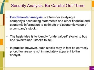
  • 4. 6-4 Security Analysis: Be Careful Out There • Fundamental analysis is a term for studying a company’s accounting statements and other financial and economic information to estimate the economic value of a company’s stock. • The basic idea is to identify “undervalued” stocks to buy and “overvalued” stocks to sell. • In practice however, such stocks may in fact be correctly priced for reasons not immediately apparent to the analyst.
  • 5. 6-5 The Dividend Discount Model • The Dividend Discount Model (DDM) is a method to estimate the value of a share of stock by discounting all expected future dividend payments. The basic DDM equation is: • In the DDM equation: – P0 = the present value of all future dividends – Dt = the dividend to be paid t years from now – k = the appropriate risk-adjusted discount rate        T T 3 3 2 2 1 0 k 1 D k 1 D k 1 D k 1 D P         
  • 6. 6-6 Example: The Dividend Discount Model • Suppose that a stock will pay three annual dividends of $200 per year, and the appropriate risk-adjusted discount rate, k, is 8%. • In this case, what is the value of the stock today?             $515.42 0.08 1 $200 0.08 1 $200 0.08 1 $200 P k 1 D k 1 D k 1 D P 3 2 0 3 3 2 2 1 0             
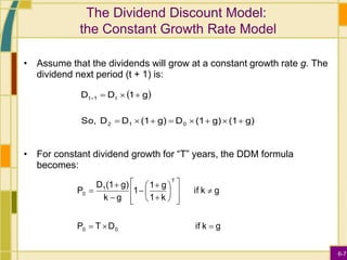
  • 7. 6-7 The Dividend Discount Model: the Constant Growth Rate Model • Assume that the dividends will grow at a constant growth rate g. The dividend next period (t + 1) is: • For constant dividend growth for “T” years, the DDM formula becomes: g k if D T P g k if k 1 g 1 1 g k g) (1 D P 0 0 T 1 0                           g) (1 g) (1 D g) (1 D D So, g 1 D D 0 1 2 t 1 t            
  • 8. 6-8 Example: The Constant Growth Rate Model • Suppose the current dividend is $10, the dividend growth rate is 10%, there will be 20 yearly dividends, and the appropriate discount rate is 8%. • What is the value of the stock, based on the constant growth rate model?   $243.86 1.08 1.10 1 .10 .08 1.10 $10 P k 1 g 1 1 g k g) (1 D P 20 0 T 0 0                                       
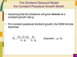
  • 9. 6-9 The Dividend Discount Model: the Constant Perpetual Growth Model. • Assuming that the dividends will grow forever at a constant growth rate g. • For constant perpetual dividend growth, the DDM formula becomes:   k) g : (Important g k D g k g 1 D P 1 0 0       
  • 10. 6-10 Example: Constant Perpetual Growth Model • Think about the electric utility industry. • In 2007, the dividend paid by the utility company, DTE Energy Co. (DTE), was $2.12. • Using D0 =$2.12, k = 6.7%, and g = 2%, calculate an estimated value for DTE. Note: the actual mid-2007 stock price of DTE was $47.81. What are the possible explanations for the difference?   $46.01 .02 .067 1.02 $2.12 P0    
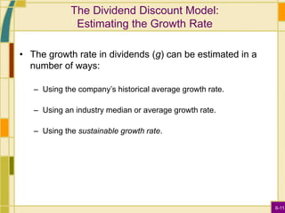
  • 11. 6-11 The Dividend Discount Model: Estimating the Growth Rate • The growth rate in dividends (g) can be estimated in a number of ways: – Using the company’s historical average growth rate. – Using an industry median or average growth rate. – Using the sustainable growth rate.
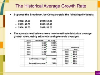
  • 12. 6-12 The Historical Average Growth Rate • Suppose the Broadway Joe Company paid the following dividends: – 2002: $1.50 2005: $1.80 – 2003: $1.70 2006: $2.00 – 2004: $1.75 2007: $2.20 • The spreadsheet below shows how to estimate historical average growth rates, using arithmetic and geometric averages. Year: Dividend: Pct. Chg: 2007 $2.20 10.00% 2006 $2.00 11.11% 2005 $1.80 2.86% Grown at 2004 $1.75 2.94% Year: 7.96%: 2003 $1.70 13.33% 2002 $1.50 2002 $1.50 2003 $1.62 2004 $1.75 8.05% 2005 $1.89 2006 $2.04 7.96% 2007 $2.20 Arithmetic Average: Geometric Average:
  • 13. 6-13 The Sustainable Growth Rate • Return on Equity (ROE) = Net Income / Equity • Payout Ratio = Proportion of earnings paid out as dividends • Retention Ratio = Proportion of earnings retained for investment Ratio) Payout - (1 ROE Ratio Retention ROE Rate Growth e Sustainabl    
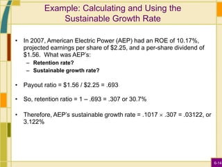
  • 14. 6-14 Example: Calculating and Using the Sustainable Growth Rate • In 2007, American Electric Power (AEP) had an ROE of 10.17%, projected earnings per share of $2.25, and a per-share dividend of $1.56. What was AEP’s: – Retention rate? – Sustainable growth rate? • Payout ratio = $1.56 / $2.25 = .693 • So, retention ratio = 1 – .693 = .307 or 30.7% • Therefore, AEP’s sustainable growth rate = .1017  .307 = .03122, or 3.122%
  • 15. 6-15 Example: Calculating and Using the Sustainable Growth Rate, Cont. • What is the value of AEP stock, using the perpetual growth model, and a discount rate of 6.7%? • The actual mid-2007 stock price of AEP was $45.41. • In this case, using the sustainable growth rate to value the stock gives a reasonably accurate estimate. • What can we say about g and k in this example?   $44.96 .03122 .067 1.03122 $1.56 P     0
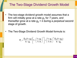
  • 16. 6-16 The Two-Stage Dividend Growth Model • The two-stage dividend growth model assumes that a firm will initially grow at a rate g1 for T years, and thereafter grow at a rate g2 < k during a perpetual second stage of growth. • The Two-Stage Dividend Growth Model formula is: 2 2 0 T 1 T 1 1 1 0 g k ) g (1 D k 1 g 1 k 1 g 1 1 g k ) g (1 D P                                0
  • 17. 6-17 Using the Two-Stage Dividend Growth Model, I. • Although the formula looks complicated, think of it as two parts: – Part 1 is the present value of the first T dividends (it is the same formula we used for the constant growth model). – Part 2 is the present value of all subsequent dividends. • So, suppose MissMolly.com has a current dividend of D0 = $5, which is expected to shrink at the rate, g1 = 10% for 5 years, but grow at the rate, g2 = 4% forever. • With a discount rate of k = 10%, what is the present value of the stock?
  • 18. 6-18 Using the Two-Stage Dividend Growth Model, II. • The total value of $46.03 is the sum of a $14.25 present value of the first five dividends, plus a $31.78 present value of all subsequent dividends. $46.03. $31.78 $14.25 0.04 0.10 0.04) $5.00(1 0.10 1 0.90 0.10 1 0.90 1 0.10) ( 0.10 ) $5.00(0.90 P g k ) g (1 D k 1 g 1 k 1 g 1 1 g k ) g (1 D P 5 5 2 2 0 T 1 T 1 1 1 0                                                                0 0
  • 19. 6-19 Example: Using the DDM to Value a Firm Experiencing “Supernormal” Growth, I. • Chain Reaction, Inc., has been growing at a phenomenal rate of 30% per year. • You believe that this rate will last for only three more years. • Then, you think the rate will drop to 10% per year. • Total dividends just paid were $5 million. • The required rate of return is 20%. • What is the total value of Chain Reaction, Inc.?
  • 20. 6-20 Example: Using the DDM to Value a Firm Experiencing “Supernormal” Growth, II. • First, calculate the total dividends over the “supernormal” growth period: • Using the long run growth rate, g, the value of all the shares at Time 3 can be calculated as: P3 = [D3 x (1 + g)] / (k – g) P3 = [$10.985 x 1.10] / (0.20 – 0.10) = $120.835 Year Total Dividend: (in $millions) 1 $5.00 x 1.30 = $6.50 2 $6.50 x 1.30 = $8.45 3 $8.45 x 1.30 = $10.985
  • 21. 6-21 Example: Using the DDM to Value a Firm Experiencing “Supernormal” Growth, III. • Therefore, to determine the present value of the firm today, we need the present value of $120.835 and the present value of the dividends paid in the first 3 years:                 million. $87.58 $69.93 $6.36 $5.87 $5.42 0.20 1 $120.835 0.20 1 $10.985 0.20 1 $8.45 0.20 1 $6.50 P k 1 P k 1 D k 1 D k 1 D P 3 3 2 3 3 3 3 2 2 1                      0 0
  • 22. 6-22 Discount Rates for Dividend Discount Models • The discount rate for a stock can be estimated using the capital asset pricing model (CAPM ). • We will discuss the CAPM in a later chapter. • However, we can estimate the discount rate for a stock using this formula: Discount rate = time value of money + risk premium = U.S. T-bill Rate + (Stock Beta x Stock Market Risk Premium) T-bill Rate: return on 90-day U.S. T-bills Stock Beta: risk relative to an average stock Stock Market Risk Premium: risk premium for an average stock
  • 23. 6-23 Observations on Dividend Discount Models, I. Constant Perpetual Growth Model: • Simple to compute • Not usable for firms that do not pay dividends • Not usable when g > k • Is sensitive to the choice of g and k • k and g may be difficult to estimate accurately. • Constant perpetual growth is often an unrealistic assumption.
  • 24. 6-24 Observations on Dividend Discount Models, II. Two-Stage Dividend Growth Model: • More realistic in that it accounts for two stages of growth • Usable when g > k in the first stage • Not usable for firms that do not pay dividends • Is sensitive to the choice of g and k • k and g may be difficult to estimate accurately.
  • 25. 6-25 Residual Income Model (RIM), I. • We have valued only companies that pay dividends. – But, there are many companies that do not pay dividends. – What about them? – It turns out that there is an elegant way to value these companies, too. • The model is called the Residual Income Model (RIM). • Major Assumption (known as the Clean Surplus Relationship, or CSR): The change in book value per share is equal to earnings per share minus dividends.
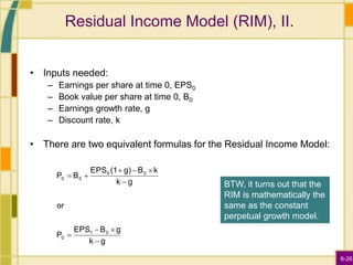
  • 26. 6-26 Residual Income Model (RIM), II. • Inputs needed: – Earnings per share at time 0, EPS0 – Book value per share at time 0, B0 – Earnings growth rate, g – Discount rate, k • There are two equivalent formulas for the Residual Income Model: g k g B EPS P or g k k B g) (1 EPS B P 0 1 0 0 0 0 0           BTW, it turns out that the RIM is mathematically the same as the constant perpetual growth model.
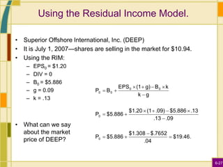
  • 27. 6-27 Using the Residual Income Model. • Superior Offshore International, Inc. (DEEP) • It is July 1, 2007—shares are selling in the market for $10.94. • Using the RIM: – EPS0 = $1.20 – DIV = 0 – B0 = $5.886 – g = 0.09 – k = .13 • What can we say about the market price of DEEP? $19.46. .04 $.7652 $1.308 $5.886 P .09 .13 .13 $5.886 .09) (1 $1.20 $5.886 P g k k B g) (1 EPS B P 0 0 0 0 0 0                  
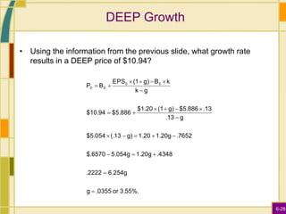
  • 28. 6-28 DEEP Growth • Using the information from the previous slide, what growth rate results in a DEEP price of $10.94? 3.55%. or .0355 g 6.254g .2222 .4348 1.20g 5.054g $.6570 .7652 1.20g 1.20 g) (.13 $5.054 g .13 .13 $5.886 g) (1 $1.20 $5.886 $10.94 g k k B g) (1 EPS B P 0 0 0 0                        
  • 29. 6-29 Price Ratio Analysis, I. • Price-earnings ratio (P/E ratio) – Current stock price divided by annual earnings per share (EPS) • Earnings yield – Inverse of the P/E ratio: earnings divided by price (E/P) • High-P/E stocks are often referred to as growth stocks, while low-P/E stocks are often referred to as value stocks.
  • 30. 6-30 Price Ratio Analysis, II. • Price-cash flow ratio (P/CF ratio) – Current stock price divided by current cash flow per share – In this context, cash flow is usually taken to be net income plus depreciation. • Most analysts agree that in examining a company’s financial performance, cash flow can be more informative than net income. • Earnings and cash flows that are far from each other may be a signal of poor quality earnings.
  • 31. 6-31 Price Ratio Analysis, III. • Price-sales ratio (P/S ratio) – Current stock price divided by annual sales per share – A high P/S ratio suggests high sales growth, while a low P/S ratio suggests sluggish sales growth. • Price-book ratio (P/B ratio) – Market value of a company’s common stock divided by its book (accounting) value of equity – A ratio bigger than 1.0 indicates that the firm is creating value for its stockholders.
  • 32. 6-32 Price/Earnings Analysis, Intel Corp. Intel Corp (INTC) - Earnings (P/E) Analysis 5-year average P/E ratio 27.30 Current EPS $.86 EPS growth rate 8.5% Expected stock price = historical P/E ratio  projected EPS $25.47 = 27.30  ($.86  1.085) Mid-2007 stock price = $24.27
  • 33. 6-33 Price/Cash Flow Analysis, Intel Corp. Intel Corp (INTC) - Cash Flow (P/CF) Analysis 5-year average P/CF ratio 14.04 Current CFPS $1.68 CFPS growth rate 7.5% Expected stock price = historical P/CF ratio  projected CFPS $25.36 = 14.04  ($1.68  1.075) Mid-2007 stock price = $24.27
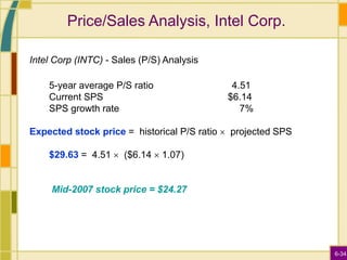
  • 34. 6-34 Price/Sales Analysis, Intel Corp. Intel Corp (INTC) - Sales (P/S) Analysis 5-year average P/S ratio 4.51 Current SPS $6.14 SPS growth rate 7% Expected stock price = historical P/S ratio  projected SPS $29.63 = 4.51  ($6.14  1.07) Mid-2007 stock price = $24.27
  • 35. 6-35 An Analysis of the McGraw-Hill Company The next few slides contain a financial analysis of the McGraw-Hill Company, using data from the Value Line Investment Survey.
  • 38. 6-38 The McGraw-Hill Company Analysis, III. • Based on the CAPM, k = 3.1% + (.80  9%) = 10.3% • Retention ratio = 1 – $.66/$2.65 = .751 • Sustainable g = .751  23% = 17.27% • Because g > k, the constant growth rate model cannot be used. (We would get a value of -$11.10 per share)
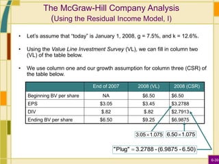
  • 39. 6-39 The McGraw-Hill Company Analysis (Using the Residual Income Model, I) • Let’s assume that “today” is January 1, 2008, g = 7.5%, and k = 12.6%. • Using the Value Line Investment Survey (VL), we can fill in column two (VL) of the table below. • We use column one and our growth assumption for column three (CSR) of the table below. End of 2007 2008 (VL) 2008 (CSR) Beginning BV per share NA $6.50 $6.50 EPS $3.05 $3.45 $3.2788 DIV $.82 $.82 $2.7913 Ending BV per share $6.50 $9.25 $6.9875 1.075 3.05 1.075 6.50 6.50) - (6.9875 - 3.2788 Plug" " 
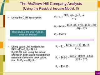
  • 40. 6-40 The McGraw-Hill Company Analysis (Using the Residual Income Model, II) • Using the CSR assumption: • Using Value Line numbers for EPS1=$3.45, B1=$9.25 B0=$6.50; and using the actual change in book value instead of an estimate of the new book value, (i.e., B1-B0 is = B0 x k) $54.73. P .075 .126 .126 $6.50 .075) (1 $3.05 $6.50 P g k k B g) (1 EPS B P 0 0 0 0 0 0                $20.23 P .075 .126 6.50) - ($9.25 $3.45 $6.50 P g k k B g) (1 EPS B P 0 0 0 0 0 0             Stock price at the time = $57.27. What can we say?
  • 42. 6-42 Useful Internet Sites • www.nyssa.org (the New York Society of Security Analysts) • www.aaii.com (the American Association of Individual Investors) • www.eva.com (Economic Value Added) • www.valueline.com (the home of the Value Line Investment Survey) • Websites for some companies analyzed in this chapter: • www.aep.com • www.americanexpress.com • www.pepsico.com • www.intel.com • www.corporate.disney.go.com • www.mcgraw-hill.com
  • 43. 6-43 Chapter Review, I. • Security Analysis: Be Careful Out There • The Dividend Discount Model – Constant Dividend Growth Rate Model – Constant Perpetual Growth – Applications of the Constant Perpetual Growth Model – The Sustainable Growth Rate
  • 44. 6-44 Chapter Review, II. • The Two-Stage Dividend Growth Model – Discount Rates for Dividend Discount Models – Observations on Dividend Discount Models • Residual Income Model (RIM) • Price Ratio Analysis – Price-Earnings Ratios – Price-Cash Flow Ratios – Price-Sales Ratios – Price-Book Ratios – Applications of Price Ratio Analysis • An Analysis of the McGraw-Hill Company