Credit scorecard
•
13 likes•6,502 views

The document provides an overview of credit scoring and scorecard development. It discusses: - The objectives of credit scoring in assessing credit risk and forecasting good/bad applicants. - The types of clients that are categorized for scoring, including good, bad, indeterminate, insufficient, excluded, and rejected. - The research objectives and challenges in building statistical models to assign risk scores and monitor model performance. - The research methodology involving data partitioning, variable binning, scorecard modeling using logistic regression, and scorecard evaluation metrics like KS, Gini, and lift.
Report
Share


Credit scorecard
- 1. Credit Scorecard BY TUHIN CHATTOPADHYAY, PH.D. 1
- 2. Introduction Credit scoring means applying a statistical model to assign a risk score to a credit application. Credit scoring techniques assess the risk in lending to a particular client. They not only identify “good” applications and “bad” applications (where negative behaviour, e.g., default, is expected) on an individual basis, but also they forecast the probability that an applicant with any given score will be “good” or “bad”. These probabilities or scores, along with other business considerations, such as expected approval rates, profit, churn, and losses, are then used as a basis for decision making. 2
- 3. Types of clients: Good and Bad: Based on the client’s number of days after the due date (days past due, DPD) and the amount past due. Indeterminate: On the border between good and bad clients. Insufficient: Clients with the very short history, which makes impossible the correct definition of dependent variable (good / bad client). Excluded: Typically clients with so wrong data as to be misleading (e.g. frauds). They are also marked as “hard bad”. Rejected: Applicants who belong to a category that will not be assessed by a model (scorecard), e.g. VIPs. 3
- 4. Business Objectives 1. Who should get credit? 2. How much credit they should receive? 3. Which operational strategies will enhance the profitability of the borrowers to the lenders? 4
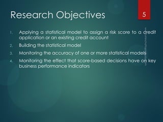
- 5. Research Objectives 1. Applying a statistical model to assign a risk score to a credit application or an existing credit account 2. Building the statistical model 3. Monitoring the accuracy of one or more statistical models 4. Monitoring the effect that score-based decisions have on key business performance indicators 5
- 6. Research Challenges To select the best model (out of Cox Proportional Hazard Model, logistic regression, decision trees, discriminant analysis, neural networks, ensemble models etc.) according to some measure of quality (Gini index, which is most widely used in Europe, KS, which is most widely used in North America and Lift) at the time of development. To monitor the quality of the model after its deployment into real business. 6
- 8. Research Methodology Step 1 • Data Partition – Training & Validation Step 2 • Interactive Grouping – Coarse Coding (“Discretizing”) Predictors Step 3 • Scorecard – Model Building (Logistic Regression) Step 4 • Scorecard Evaluation – KS, LC, Gini, Lift Step 5 • Reject Inference – Fuzzy, Hard Cutoff and Parcelling Step 6 • Data Partition (2) – Training, Testing & Validation Step 7 • Research Design – 3 Experiments Step 8 • Model Building – Cox, Discriminant, CART, LR, NN & Ensembles Step 9 • Model Comparison – ROC, AUR, AIC, BIC, Gini, Cumulative Lift Step 10 • Monitoring the Scorecard – Vintage Analysis & Population Analysis 8
- 10. 10
- 11. 11
- 12. 12
- 14. Tabulation of Data All borrowers should be marked in the target column as “Good” or “Bad” by a certain rule. For example: all the borrowers to pay in 30 days, are “Good”, but borrowers with a delay of more than 90 days are marked as “Bad”. 14
- 15. Tabulation of Data Historical data should include a set of characteristics and a target variable. All of scorecard development methods quantify the relationship between the characteristics (input columns) and “Good/Bad” performance (target column). 15
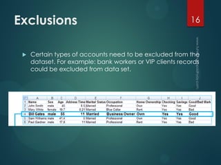
- 16. Exclusions Certain types of accounts need to be excluded from the dataset. For example: bank workers or VIP clients records could be excluded from data set. 16
- 19. Those characteristics, whose usage is not reasonable, should be marked with caution. For example: on the picture you can see that the “Good/ Bad” distribution does not depend on the Home Ownership characteristics. Don’t Remove but Be Cautious!19
- 20. Step 1: Partition the Data Training data set: Used for preliminary model fitting. Validation data set: Used to prevent a modelling node from overfitting the training data and to compare models. Test data set: used for a final assessment of the model. Training: 70/80 & Validation: 30/20 20
- 21. Step 2: Interactive Grouping – Coarse Coding (“Discretizing”) Predictors/ Binning Binning means the process of transforming a numeric characteristic into a categorical one as well as re-grouping and consolidating categorical characteristics. Initial automatic grouping of input variables into bins to provide optimal splits. Regroup the variables through an interactive interface. Screen or select variables. 21
- 22. Why Binning is Required? Increases scorecard stability: some characteristic values can rarely occur, and will lead to instability if not grouped together. Improves quality: grouping of similar attributes with similar predictive strengths will increase scorecard accuracy. Allows to understand logical trends of “Good/Bad” deviations for each characteristic. Prevents scorecard impairment otherwise possible due to seldom reversal patterns and extreme values. Prevents overfitting(overtraining) possible with numerical variables. 22
- 23. Automatic Binning The most widely used automatic binning algorithm is Chi- merge. Chi-merge is a process of dividing into intervals (bins) in the way that neighbouring bins will differ from each other as much as possible in the ratio of “Good” and “Bad” records in them. For visual cross-verification of automatic binning results one can use WOE values 23
- 24. Interactive Grouping @ SAS E-Miner Initial automatic grouping of input variables into bins to provide optimal splits. Regroup the variables through an interactive interface. Screen or select variables. 24
- 25. 25
- 26. Information Value (IV) IV is used to evaluate a characteristic’s overall predictive power i.e. the characteristic’s ability to separate between good and bad loans. < 0.02 is unpredictive 0.02 - 0.10 is weakly predictive. 0.10 and 0.30 is moderately predictive. > 0.30 is strongly predictive. Let’s Reject if the variable’s IV < 0.10. Here L is the number of attributes for the characteristic variable. 26
- 27. Weight of Evidence (WOE) Weight of evidence (WOE) measures the strength of an attribute of a characteristic in differentiating good and bad accounts. Weight of evidence is based on the proportion of good applicants to bad applicants at each group level. Negative values indicate that a particular grouping is isolating a higher proportion of bad applicants than good applicants i.e. negative WOE values are worse in the sense that applicants in that group present a greater credit risk. For each group i of a characteristic WOE is calculated as follows: 27
- 28. Weight of Evidence Coding 28
- 29. 29
- 30. Sharply-varied and illogical WOE graph after automatic binning 30
- 31. Manual Specification of Cut-Off Value @ Split Bin Window 31
- 32. Merge Bin 32
- 33. New Group 33
- 34. 34
- 35. Smooth and logical WOE decline after manual correction 35
- 36. Step 3: Scorecard 36
- 37. Next Step: Scorecard 37
- 38. Decision from Scorecard Note: A scorecard is scaled with the Odds, Scorecard Points and Points to Double the Odds properties. 38
- 40. Logistic Regression The regression coefficients are used to scale the scorecard. Scaling a scorecard refers to making the scorecard conform to a particular range of scores. Logistic regression yields prediction probabilities for whether or not a particular outcome (e.g., Bad Credit) will occur. Logistic regression models are linear models, in that the logit- transformed prediction probability is a linear function of the predictor variable values. Thus, a final score card model derived in this manner has the desirable quality that the final credit score (credit risk) is a linear function of the predictors, and with some additional transformations applied to the model parameter, a simple linear function of scores that can be associated with each predictor class value after coarse coding. So the final credit score is then a simple sum of individual score values that can be taken from the scorecard. 40
- 41. Logistic Regression Given a vector of application characteristics x, the probability of default p is related to vector x by the relationship • where coefficients wi represent the importance of specific loan application characteristic coefficients xi in the logistic regression. • Three types: Forward, Backward and Stepwise • Coefficients wi are obtained by using maximum likelihood estimation (MLE). 41
- 42. Regression Coefficients from the Scorecard Node 42
- 43. Score-Points Scaling For each attribute, its Weight of Evidence and the regression coefficient of its characteristic now could be multiplied to give the score points of the attribute. An applicant’s total score would then be proportional to the logarithm of the predicted bad/good odds of that applicant. 43
- 44. Scaling a Scorecard Objectives: 1. To determine the odds at a certain score. 2. To determine the points required to double the odds. 44
- 45. Score-Points Scaling Mechanism Score points are commonly scaled linearly to take more friendly (integer) values and conform to industry or company standards. We scale the points such that a total score of 600 points corresponds to good/bad odds of 50 to 1 and an increase of the score of 20 points corresponds to a doubling of the good/bad odds. The scorecard points are scaled so that a total score of 600 corresponds to good:bad odds of 30:1 and that an increase of 20 points corresponds to a doubling of the good:bad odds. 45
- 46. For the derivation of the scaling rule that transforms the score points of each attribute, the calculation is as follows: Score = The scaling rule is implemented in the Properties panel of the Scorecard node: Score-Points Scaling Calculation46
- 47. 47
- 48. 48
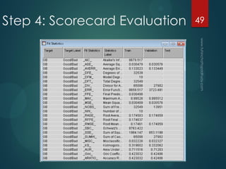
- 49. Step 4: Scorecard Evaluation 49
- 50. Distribution of Functions, KS A score of around 2.5 or smaller has a population including approximately 30% of good clients and 70% of bad clients. 50
- 51. In this graph, the X axis shows the credit score values (sums), and the Y axis denotes the cumulative proportions of observations in each outcome class (Good Credit vs. Bad Credit) in the hold-out sample. The further apart are the two lines, the greater is the degree of differentiation between the Good Credit and Bad Credit cases in the hold-out sample, and thus, the better (more accurate) is the model. 51
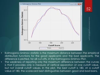
- 52. • Kolmogorov-Smirnov statistic is the maximum distance between the empirical distribution functions for the good applicants and the bad applicants. The difference is plotted, for all cut-offs, in the Kolmogorov-Smirnov Plot. • The weakness of reporting only the maximum difference between the curves is that it provides only a measure of vertical separation at one cutoff value, but not overall cutoff values. In the plot, the best cutoff is 180. At a cutoff value of 180, the scorecard best distinguishes between good and bad loans. 52
- 53. Lorenz Curve (LC) By rejecting 20% of good clients, we reject almost 60% of bad clients at the same time. 53
- 54. Receiver Operating Characteristic (ROC) Curve Illustrates the performance of a binary classifier system as its discrimination threshold is varied. The curve is created by plotting the true positive rate (TPR) against the false positive rate (FPR) at various threshold settings. The true-positive rate is also known as sensitivity or recall. The false-positive rate is calculated as (1 - specificity). 54
- 56. Area Under the Receiver operating characteristic curve (AUR) The closer the curve follows the left-hand border and then the top border of the ROC space, the more accurate the test. The AUR measures the area below each of the curves. A scorecard that is no better than random selection has an AUR value equal to 0.50. The maximum value of the AUR is 1.0. 56
- 57. Akaike Information Criterion (AIC) We start with a set of candidate models, and then find the models' corresponding AIC values. There will almost always be information lost due to using a candidate model to represent the "true" model (i.e. the process that generates the data). We wish to select, from among the candidate models, the model that minimizes the information loss. Given a set of candidate models for the data, the preferred model is the one with the minimum AIC value. Suppose that there are R candidate models. Denote the AIC values of those models by AIC1, AIC2, AIC3, …, AICR. Let AICmin be the minimum of those values. Then exp((AICmin − AICi)/2) can be interpreted as the relative probability that the ith model minimizes the (estimated) information loss. As an example, suppose that there are three candidate models, whose AIC values are 100, 102, and 110. Then the second model is exp((100 − 102)/2) = 0.368 times as probable as the first model to minimize the information loss. Similarly, the third model is exp((100 − 110)/2) = 0.007 times as probable as the first model to minimize the information loss. The quantity exp((AICmin − AICi)/2) is the relative likelihood of model i. 57
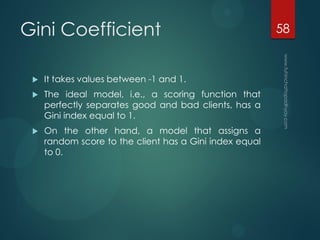
- 58. Gini Coefficient It takes values between -1 and 1. The ideal model, i.e., a scoring function that perfectly separates good and bad clients, has a Gini index equal to 1. On the other hand, a model that assigns a random score to the client has a Gini index equal to 0. 58
- 59. Bayesian Information Criterion (BIC) or Schwarz Criterion (SBC, SBIC) When picking from several models, the one with the lowest BIC is preferred. The strength of the evidence against the model with the higher BIC value can be summarized as follows: ΔBIC Evidence against higher BIC 0 to 2 Not worth more than a bare mention 2 to 6 Positive 6 to 10 Strong >10 Very Strong 59
- 60. Calculation of Lift Ratio Assume that we have a score of 1000 clients, of which 50 are bad. The proportion of bad clients is 5%. Sort customers according to score and split into ten groups, i.e., divide it by deciles of score. In each group, in our case around 100 clients, then count bad clients. This will get their share in the group (Bad Rate). Absolute Lift in each group is then given by the ratio of the share of bad clients in the group to the proportion of bad clients in total. 60
- 61. Absolute and Cumulative Lift61
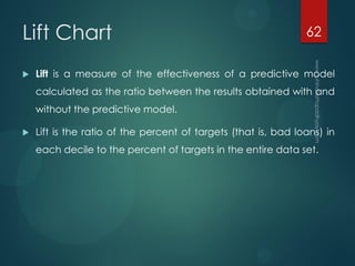
- 62. Lift Chart Lift is a measure of the effectiveness of a predictive model calculated as the ratio between the results obtained with and without the predictive model. Lift is the ratio of the percent of targets (that is, bad loans) in each decile to the percent of targets in the entire data set. 62
- 63. Cumulative lift chart Cumulative lift is the cumulative ratio of the percent of targets (i.e., bad loans) up to the decile of interest to the percent of targets in the entire data set. The Cumulative Lift Chart shows you the lift factor of how many times it is better to use a model in contrast to not using a model. The x-coordinate of the chart shows the percentage of the cumulated number of sorted data records of the current model. The data records are sorted in descending order by the confidence that the model assigns to a prediction of the selected value of the target field. The y-coordinate of the Cumulative Lift Chart shows the cumulated lift factor or the cumulative average percentage of the selected target field value. 63
- 64. Cumulative Lift Chart for a Single Model 64
- 65. Step 5: Reject Inference How to deal with the inherent bias when modelling is based on a training dataset consisting only of those previous applicants for whom the actual performance (Good Credit vs. Bad Credit) has been observed; There are likely another significant number of previous applicants, that had been rejected and for whom final "credit performance" was never observed. How to include those previous applicants in the modelling, in order to make the predictive model more accurate and robust (and less biased), and applicable also to those individuals. 65
- 66. Benefits of Reject Inference 66
- 67. Inclusion of Rejects Data Drag and drop the REJECTS data source onto the diagram and connect it with the Reject Inference node. Make sure that the REJECTS data source is defined as a SCORE data set. 67
- 68. Inference Methods 1. Fuzzy: Allocates weight to observations in the augmented data set. The weight reflects the observation's tendency to be “good” or “bad”. 2. Hard Cutoff: Classifies observations as either good or bad based on a cutoff score. 3. Parceling: Distributes binned, scored rejected applicants into either a good bin or a bad bin. 68
- 69. Rejection Rate Specify a value for the Rejection Rate property when using either the Hard Cutoff or Parceling inference method. The Rejection Rate is used as a frequency variable. The rate of bad applicants is defined as the number of bad applicants divided by the total number of applicants. The value for the Rejection Rate property must be a real number between 0.0001 and 1. The default value is 0.3. 69
- 70. Fuzzy The partial classification information is based on the probability of being good or bad based on the model built with the CS_ACCEPTS data set that is applied to the CS_REJECTS data set. Fuzzy classification multiplies these probabilities by the user- specified Reject Rate parameter to form frequency variables. This results in two observations for each observation in the Rejects data. Let p(good) be the probability that an observation represents a good applicant and p(bad) be the probability that an observation represents a bad applicant. The first observation has a frequency variable defined as (Reject Rate)*p(good) and a target variable of 0. The second observation has a frequency variable defined as (Reject Rate)*p(bad) and a target value of 1. Fuzzy is the default inference method. 70
- 71. Parceling Distribution is based on the expected bad rates that are calculated from the scores from the logistic regression model. The parameters that must be defined for parcelling vary according to the Score Range method that one selects in the Parceling properties group. All parcelling classifications require to specify the Rejection Rate, Score Range Method, Min Score, Max Score, and Score Buckets properties. 71
- 72. Parceling Properties (Score Buckets) 1. Score Range Method: To specify how you want to define the range of scores to be bucketed. Accepts — Distributes the rejected applicants into equal-sized buckets based on the score range of the CS_ACCEPTS data set. Rejects — Distributes the rejected applicants into equal-sized buckets based on the score range of the CS_REJECTS data set. Scorecard — Distributes the rejected applicants into equal-sized buckets based on the score range that is output by the augmented data set. Manual — Distributes the rejected applicants into equal-sized buckets based on the range that you input. 2. Score Buckets: To specify the number of buckets that you want to use to parcel the data set into during attribute classification. Permissible Score Buckets property values are integers between 1 and 100. The default setting for the Score Buckets property is 25. 72
- 73. Step 6: Partition the Data Training data set: used for preliminary model fitting. Validation data set: used to prevent a modelling node from overfitting the training data and to compare models. Test data set: used for a final assessment of the model. 60% for training, 20% for validation and 20% for testing 73
- 74. Step 7: Experimental Design Experiment 1: Data set without any variable transformations or variable reduction. Experiment 2: Data set without any variable transformations, but eliminated the variables that are weakly correlated with the target variable. Experiment 3: With variable transformations - such as bucketing for variables that had highly skewed distributions etc. 74
- 75. Statistical Design In each experiment, eight different data mining tools: neural networks, decision trees, logistic regression, discriminant analysis, Cox Proportional Hazard Model and stochastic gradient boosting, random forest, SVM will be employed. Finally, the eight tools will be combined into an ensemble model to increase the reliability of the classification accuracy by improving the stability of the three disparate non-linear models. The ensemble model averages the posterior probabilities for class target variable BAD from the six tools. Given the posterior probabilities, each case can be classified into the most probable class. So there will be a total of nine comparisons in each of the three experiments. 75
- 76. Step 8: Model Development 1. Cox Proportional Hazard Model: Cox model (for short) predicts the probability of failure, default, or "termination" of an outcome within a specific time interval. An alternative and refinement to logistic regression in particular when "life-times" for credit performance (until default, early pay-off, etc.) are available in the training data. 2. Artificial Neural Networks 3. Stochastic Gradient Boosting 4. Discriminant Analysis 5. Logistic Regression 6. Decision Tree 7. Random Forest 8. SVM 76
- 77. Flowchart @ SAS E-Miner 77
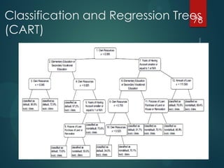
- 78. Classification and Regression Trees (CART) 78
- 79. Why Decision Tree? A decision tree may outperform a scorecard in terms of predictive accuracy because, unlike the scorecard, it detects and exploits interactions between characteristics. In a decision tree model, each answer that an applicant gives determines what question is asked next. If the age of an applicant is, for example, greater than 50, the model may suggest granting a credit without any further questions because the average bad rate of that segment of applications is sufficiently low. If, on the other extreme, the age of the applicant is below 25, the model may suggest asking next about time of employment. Then, credit might be granted only to those who have exceeded 24 months of employment, because only in that subsegment of younger adults is the average bad rate sufficiently low. A decision tree model consists of a set of “if ... then ... else” rules that are still quite straightforward to apply. The decision rules also are easy to understand, perhaps even more so than a decision rule that is based on a total score made up of many components. 79
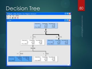
- 80. Decision Tree 80
- 82. Step 9: Model Comparison 82
- 83. Model Comparison with Ensemble 83
- 84. The AUCs of benchmark model and new models 84
- 85. Cumulative Lift Chart for Multiple Models 85
- 86. Stability and Performance of the Models 86
- 87. 87
- 88. 88
- 89. Step 10: Monitoring the Scorecard Population Stability Reports: To capture and track changes in the population of applications (the composition of the applicant pool with respect to the predictors) Scorecard Performance: The predictions from the scorecard may become increasingly inaccurate. Thus, the accuracy of the predictions from the model must be tracked, to determine when a model should be updated or discarded (and when a new model should be built). Vintage Analysis (Delinquency Reports): The actual observed rate of default (Bad Credit) may change over time (e.g., due to economic conditions). 89
- 90. Population Stability Reports Population stability reports are used for monitoring trends in credit scoring. Over time, economic factors and changes within a financial institution such as marketing campaigns or credit offers can affect the credit scoring process. The purpose of a population stability report is to detect shifts or trends within the credit applicant pool and factors related to these. With the information from the population stability report, the institution can update credit scorecards as well as make changes to better suite the needs of its customer base. The report may contain items such as the mean score or a comparison of actual and expected distribution of scores from the scorecard, a comparison of actual versus expected distributions of customer characteristics used in for scoring, approval rates, etc. 90
- 91. Vintage Analysis A vintage is a group of credit accounts that all originated within a specific time period, usually a year. Vintage analysis is used in credit scoring and refers to the process of monitoring groups of accounts and comparing performance across past groups. The comparisons take place at similar loan ages, allowing for the detection of deviation from past performance. Typically, a graphical representation is used for this purpose, such as one showing the relationship between months on the books and the percentage of delinquent accounts across multiple vintages. 91
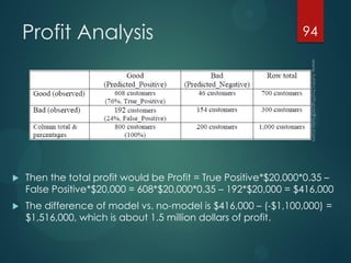
- 92. Last but not the Least: Profit Analysis Correct Decision: The bank predicts that a customer’s credit is in good standing (and hence would obtain the loan), and the customer is indeed has good credit. Bad Decision: If the model or the manager makes a false prediction that the customer’s credit is in good standing, yet the opposite is true, then the bank will result in a unit loss. 92
- 93. Profit Analysis Assume that a correct decision of the bank would result in 35% of the profit at the end of a specific period, say 3–5 years. In the second column of the matrix, the bank predicted that the customer’s credit is not in good standing and declined the loan. Hence there is no gain or loss in the decision. The data has 70% credit- worthy (good) customers and 30% not-credit-worthy (bad) customers. A manager without any model that gives everybody the loan would result in the following negative profit per customer: (700*0.35- 300*1.00)/1000 = -55/1000 = -0.055 unit loss. This number (-0.055 unit loss) may seem small. But if the average of the load is $20,000 for this population (n = 1000), then the total loss will be (-0.055 unit loss)*($20,000 per unit per customer)*(1,000 customers) = - $1,100,000, which would be a whopping one million and one hundred thousand dollar loss. 93
- 94. Profit Analysis Then the total profit would be Profit = True Positive*$20,000*0.35 – False Positive*$20,000 = 608*$20,000*0.35 – 192*$20,000 = $416,000 The difference of model vs. no-model is $416,000 – (-$1,100,000) = $1,516,000, which is about 1.5 million dollars of profit. 94
- 95. 95
- 96. The table shows that the Neural Network achieves the best profit at 5% cutoff and the Regression achieves the best profit at the 5% or 10% cutoff. In short, if we use the Neural Network model to select the top 5% of the customers, then the model would produce a Total Profit of 5.25 units for each unit of the investment in the Holdout data (n=300). Assume that we have a new population of 1,000 customers with average loan of $20,000. The Neural Network model would select the top 5% of the customer and results in a total profit of quite a bit of money indeed. Total Profit = Mean Profit*Cutoff*Population Size = 0.35*0.05*1000*$20,000 = $350,000 96
- 97. The Road Ahead 97
- 98. References 1. Chengwei Yuan (2014), Classification of Bad Accounts in Credit Card Industry. 2. Chamont Wang, Profit Analysis of the German Credit Data 3. Joshua White and Scott Baugess (2015) Qualified Residential Mortgage: Background Data Analysis on Credit Risk Retention. Division of Economic and Risk Analysis (DERA). U.S. Securities and Exchange Commission 4. Jozef Zurada & Martin Zurada (University of Louisville). How Secure Are “Good Loans”: Validating Loan-Granting Decisions And Predicting Default Rates On Consumer Loans. The Review of Business Information Systems, 2002, Volume 6, Number 3 5. Kocenda, Evzen and Vojtek, Martin, Default Predictors in Retail Credit Scoring: Evidence from Czech Banking Data (April 18, 2011). William Davidson Institute Working Paper No. 1015. 98
- 99. 4. Martin ŘEZÁČ & František ŘEZÁČ (Masaryk University, Brno, Czech Republic) How to Measure the Quality of Credit Scoring Models. Finance a úvěr-Czech Journal of Economics and Finance, 61, 2011, no. 5 5. SAS Institute Inc. 2012. Developing Credit Scorecards Using Credit Scoring for SAS® Enterprise Miner™ 12.1. Cary, NC: SAS Institute Inc. 6. Statistical Applications of Credit Scoring http://www.statsoft.com/Textbook/Credit-Scoring 7. William H. Greene (1992) A Statistical Model for Credit Scoring New York University. 99
- 100. 10 0