Data Reduction
- 1. Data Reduction: Attribute Subset Selection and Data Cube Aggregation PREPARED BY: RAJAN SHAH DMBI SVIT, VASAD
- 2. Data Reduction Data Reduction techniques can be applied to obtain a reduced representation of the data set that is much smaller in volume, yet closely maintains the integrity of the original data. That, is, Mining on the reduced data set should be more efficient yet produce the same analytical results.
- 3. Data Reduction Strategies 1. Dimensionality Reduction 2. Numerosity Reduction 3. Data Compression
- 4. Dimensionality Reduction Dimensionality Reduction is the process of reducing the number of random variables or attributes under consideration. Attribute Subset Selection is a method of dimensionality reduction in which irrelevant, weakly relevant, or redundant attributes are detected and removed.
- 5. Numerosity Reduction These techniques replace the original data volume by alternative, smaller forms of data representation. May be Parametric or Non- Parametric. Parametric Methods: A model is used to estimate the data, so that only the data parameters need to be restored and not the actual data. It assumes that the data fits some model estimates model parameters. Examples: Regression and Log-Linear Models.
- 6. Cont… Non-Parametric Methods: Do not assume the data and are used for storing reduced representations of the data which includes Histograms, Clustering, Sampling and Data Cube Aggregation.
- 7. Data Compression Transformations are applied so as to obtain a “COMPRESSED” representation of the original data. If the original data can be reconstructed from the compressed one without loss of any information, it is called Lossless Data Reduction, else it is called Lossy Data Reduction.
- 8. Attribute Subset Selection Also known as Feature Selection, which is a procedure to find a subset of features (relevant to mining task) to produce “better” model for given dataset, i.e. removal of redundant data from the data set which can slow down the mining process. AIM: To find a minimum set of attributes such that the mining process results are as close as possible to the original distribution obtained using all attributes.
- 9. Advantages Mining on Reduced set of Attributes result in reduced number of attributes and thus helping to make patterns easier to detect and understand.
- 10. How To Find a GOOD Subset? For n attributes, there are 2n possible subsets and thus the methods applied are “greedy” in that, while searching through attribute space, they always make what looks to be the local best choice assuming that it will lead to the global optimal result. The BEST and WORST attributes are determined using tests of Statistical significance assuming the attributes are independent of each other. Information Gain can be used to evaluate attributes.
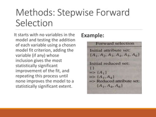
- 11. Methods: Stepwise Forward Selection It starts with no variables in the model and testing the addition of each variable using a chosen model fit criterion, adding the variable (if any) whose inclusion gives the most statistically significant improvement of the fit, and repeating this process until none improves the model to a statistically significant extent. Example:
- 12. Stepwise Backward Elimination It involves starting with all candidate variables, testing the deletion of each variable using a chosen model fit criterion, deleting the variable (if any) whose loss gives the most statistically insignificant deterioration of the model fit, and repeating this process until no further variables can be deleted without a statistically significant loss of fit. Example:
- 13. Bi-Directional Selection and Elimination The stepwise forward selection and backward elimination methods can be combined so that, at each step, the procedure selects the best attribute and removes the worst from among the remaining attributes. Example: Suppose, when A1(best) is selected, at the same time A2(worst) is eliminated. And similarly when A4 is selected, A5 gets eliminated and when A6 is selected, A3 is eliminated, thus forming the reduced set {A1, A4, A6}.
- 14. Decision Tree Induction Decision Tree Induction constructs a flowchart where each internal non-leaf node denotes a test on an attribute, each branch corresponds to an outcome of the test, and each external leaf node denotes class- prediction. At each node, the algorithm chooses the “best” attribute to partition the data into individual classes. All the attributes that do not appear in the tree are assumed to be irrelevant, while the attributes that belong to the tree form the reduced data set.
- 15. Cont…
- 16. Data Cube Aggregation A data cube is generally used to easily interpret data. It is especially useful when representing data together with dimensions as certain measures of business requirements. A cube's every dimension represents certain characteristic of the database. Data Cubes store multidimensional aggregated information. Data cubes provide fast access to precomputed, summarized data, thereby benefiting online analytical processing (OLAP) as well as data mining.
- 17. Categories of Data Cube Dimensions: Represents categories of data such as time or location. Each dimension includes different levels of categories. Example:
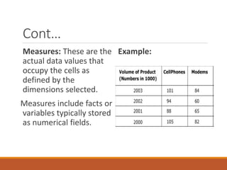
- 18. Cont… Measures: These are the actual data values that occupy the cells as defined by the dimensions selected. Measures include facts or variables typically stored as numerical fields. Example:
- 19. Cont… Example: For the data set of employees with their dept_id, salary, data cube can be used to aggregate the data so that resulting data summarizes the total salary corresponding to the dept_id. The Resulting data is smaller in volume, without loss of information necessary for analysis task.
- 20. Cont… Concept Hierarchies may exist for each attribute, allowing the analysis of data at multiple abstraction levels. The Cube created at the lowest abstraction level is called– Base Cuboid. The Cube created at the highest abstraction level is called– Apex Cuboid. Data cube can be 2-D, 3-D or higher dimension. When replying to data mining requests, the smallest available cuboid relevant to the given task should be used.
- 21. Example


