


Deep Learning for Text (Text Mining) LSTM
- 1. Deep Learning for Text Neural Network,RNN, LSTM CHIEN CHIN CHEN Deep Learning with Python - Manning Publications François Chollet, 2017
- 2. Preface This subject is intended as a primer for those with no experience in neural networks. ◦ We will not go into the math of the underlying algorithm, backpropagation. Instead, we first present basic components of neural networks. ◦ Neurons, fully connected networks. And then talk about some advanced network structure. ◦ Embedding layers, recurrent neural networks, long short-term memory networks. Examples of IMDB review sentiment analysis will be provided to practice these well-known networks. 2
- 3. Anatomy of a Neural Network (1/4) What is a neural network? ◦ A network normally consists of layers and weights. ◦ Analyze the input (data features) to predict or estimate something … Input layer … … hidden layerS output layer 年齡 性別 是否透過iPhone瀏覽 年薪 房車 休旅車 跑車 36 1 1 80 0.58 0.14 0.28 3
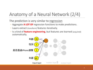
- 4. Anatomy of a Neural Network (2/4) The prediction is very similar to regression ◦ Aggregate A LOT OF regression functions to make predictions. ◦ Layers extract (transform) features iteratively. ◦ Is a kind of feature engineering, but features are learned (acquired) automatically. … Input layer … … hidden layerS output layer 年齡 性別 是否透過iPhone瀏覽 年薪 36 1 1 80 0.71 0.43 -0.22 0.71 0.68 4
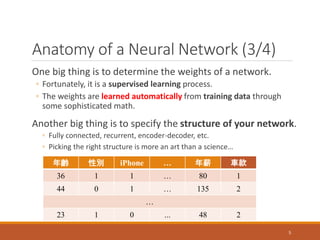
- 5. Anatomy of a Neural Network (3/4) One big thing is to determine the weights of a network. ◦ Fortunately, it is a supervised learning process. ◦ The weights are learned automatically from training data through some sophisticated math. Another big thing is to specify the structure of your network. ◦ Fully connected, recurrent, encoder-decoder, etc. ◦ Picking the right structure is more an art than a science… 年齡 性別 iPhone … 年薪 車款 36 1 1 … 80 1 44 0 1 … 135 2 … 23 1 0 ... 48 2 5
- 6. Anatomy of a Neural Network (4/4) The overview of neural network learning: Network structure & weights Training data Evaluate how good the network is Sophisticated math used to adjust weights 6
- 7. IMDB Sentiment Dataset The dataset comes packaged with Keras. ◦ Has been preprocessed – the reviews (sequences of words) have been turned into sequence of integers (unique word ids). 50,000 polarized reviews. ◦ 25,000 for training and 25,000 for testing. ◦ Each set consists of 50% negative and 50% positive reviews. The sentiment detection task is simply a binary classification. ◦ Positive/negative reviews. 7
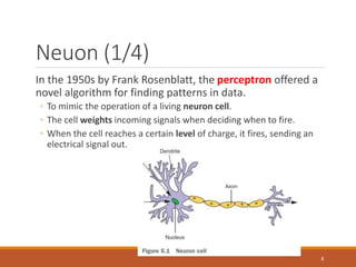
- 8. Neuon (1/4) In the 1950s by Frank Rosenblatt, the perceptron offered a novel algorithm for finding patterns in data. ◦ To mimic the operation of a living neuron cell. ◦ The cell weights incoming signals when deciding when to fire. ◦ When the cell reaches a certain level of charge, it fires, sending an electrical signal out. 8
- 9. Neuon (2/4) Rosenblatt’s research was to teach a machine to recognize images. ◦ E.g., hot dog/not hot dog. Features of the input image were each a small subsection of the image. A weight was assigned to each feature, to measure the importance of each feature. ? Activation function: once the weighted sum is above a certain threshold, the perceptron outputs 1!! Here, the activation function is a step function. 9
- 10. Neuon (3/4) The reason for having the bias is that you need the perceptron to be resilient to inputs of all zeros. ◦ Sometime, you need your network not to output 0 when facing inputs of 0. ◦ With this bias, you have no problem. Of course, the weights will be learned by training examples; rather than manually assign!! 10
- 11. Neuon (4/4) The base unit of neural networks is the neuron!! Some people regard perceptron is a special case of neuron that uses step function as the activation function. Many prefer using continuously differentiable nonlinear function (e.g., sigmoid) as the activation function of neuron. ◦ To be able to model difficult problems. ◦ Allowing backpropagation training. Sigmoid function: 𝑆(𝑥) = 1 1 + 𝑒−𝑥 11
- 12. Fully Connected Network (1/11) The most popular neural network structure ◦ Each input element has a connection to every neuron in the next layer. ◦ And the outputs of layer k become the input of layer k+1, and so on. … Input layer … … hidden layerS output layer 12
- 13. Fully Connected Network (2/11) To process text information, we need to vectorize the input text. ◦ Multi-hot encoding/Embedding layer Let’s start with the multi-hot encoding and a simple three-layer structure. … Input layer … … hidden layerS output layer term1 term2 term|V| Positive or not? 0 1 1 0 0.14 term3 13
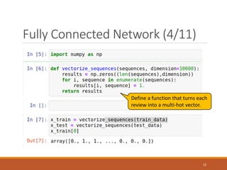
- 14. Fully Connected Network (3/11) Loading the IMDB dataset, only returning the top 10,000 most frequently occurring words 14
- 15. Fully Connected Network (4/11) Define a function that turns each review into a multi-hot vector. 15
- 16. Fully Connected Network (5/11) 16
- 17. Fully Connected Network (6/11) Loss function: a.k.a. objective function, measures how well the learned model (weights) fits the training data. ◦ Binary crossentropy for binary classification problem ◦ yi: 1/0, the target value of i-th training example. ◦ 𝑦𝑖: the output of the model regarding i-th training example. ◦ Categorical crossentropy for multi-class classification problem. ◦ MSE for regression problem. 17
- 18. Fully Connected Network (7/11) Optimizer: approach to adjust (update) network weights. ◦ SGD, RMSprop, Adam, … etc; most of them are based on gradient descent. 18
- 19. Fully Connected Network (8/11) We split training data into training/validation sets. ◦ The validation set is used to search appropriate hyper-parameters. ◦ E.g., activation function, number of hidden nodes, number of layers …. 19
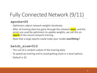
- 20. Fully Connected Network (9/11) epochs=20 ◦ Optimizers adjust network weights iteratively. ◦ After all training data has gone through the network once, and the errors are used by optimizers to update weights, we call this an epoch of the neural network training. ◦ Note that a large epochs could make your model overfitting!! batch_size=512 ◦ The size of a random subset of the training data. ◦ To speed up training and to avoid getting stuck in a local optima. ◦ Default is 32. 20
- 21. Fully Connected Network (10/11) Example of overfitting the training dataset 21
- 22. Fully Connected Network (11/11) 22
- 23. Embedding Layer (1/10) The dimension of multi-hot vectors is too high, and too sparse. ◦ In the last example, vector dimension is 10,000!! Word embeddings are low-dimensional, and dense vectors. ◦ The dimension of word embeddings is usually less than 1,000. ◦ Word embeddings are learned from data. ◦ To make synonyms embedded into similar (close) vectors. Two ways to obtain word embeddings: ◦ Learn word embeddings jointly with the task you care about (e.g., the IMDB sentiment analysis). ◦ Using pre-trained word embeddings (e.g., Word2Vec). Note that it is good to learn task-specific embeddings if you have plenty of task-specific data; pre-trained embeddings sometimes would be too general to specific tasks. 23
- 24. Embedding Layer (2/10) The following example shows how to add embedding layers into your neural network. One difficulty – different review lengths; but the size of network inputs needs to be fixed!! ◦ Here, we simply examine the first 100 words of each review. 24
- 26. Embedding Layer (4/10) 1 0 0 … … Input: 1 14 22 … 1067 2.5 0.7 … 1.8 3.7 0.8 … 0.1 … 1’s embedding 1067’s embedding 2.5 0.7 … 0.1 flatten … 2.5 0.7 1.8 26
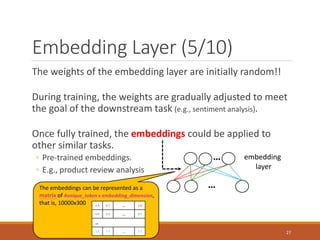
- 27. Embedding Layer (5/10) The weights of the embedding layer are initially random!! During training, the weights are gradually adjusted to meet the goal of the downstream task (e.g., sentiment analysis). Once fully trained, the embeddings could be applied to other similar tasks. ◦ Pre-trained embeddings. ◦ E.g., product review analysis … … embedding layer The embeddings can be represented as a matrix of #unique_token x embedding_dimension, that is, 10000x300 2.5 0.7 … 1.8 0.4 3.3 … 0.7 … 1.2 1.7 … 2.2 27
- 28. Embedding Layer (6/10) When training word embeddings, the embedding quality depends on the size of your training set. ◦ If you have little training data, you might not be able to learn appropriate task-specific embeddings. An alternative is to load embedding vectors from a precomputed embedding space that captures generic language structures. ◦ Remember Word2Vec? Below, we demonstrate how to load Word2Vec word embedding into a Keras Embedding layer. 28
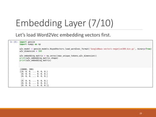
- 29. Embedding Layer (7/10) Let’s load Word2Vec embedding vectors first. 29
- 30. Embedding Layer (8/10) Next, build up the embedding matrix that we will load into an Embedding layer for our neural network model. Not every word can be found in a pre-trained model!! Zero embedding if a word is unknown to Word2Vec!! 30
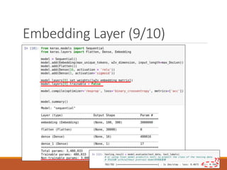
- 32. Embedding Layer (10/10) When lots of training data is available, models with a task- specific embedding are generally more powerful (accurate) than those with pre-trained embeddings. ◦ In this example, we train models with 25,000 reviews. ◦ That is why the model with pre-trained embeddings is inferior to the first task-specific embedding model. ◦ Self-practice: randomly select 200 reviews for training, and compare the two models. 32
- 33. Recurrent Neural Networks (1/6) A network structure useful for sequential data. ◦ E.g., time series and TEXT – token by token!! Offering a kind of memory mechanism that helps process data sequentially. ◦ Like human being, enable the model to observe review tokens one by one, and gradually realize the emotion of the author. By contrast, the neural networks seen so far keep no state between inputs. ◦ Each input is processed independently. 33
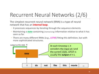
- 34. Recurrent Neural Networks (2/6) The simplest recurrent neural network (RNN) is a type of neural network that has an internal loop. ◦ It processes sequences by iterating through the sequence elements ◦ Maintaining a state containing (memorizing) information relative to what it has seen so far. ◦ There are many different RNNs (e.g., LSTM) fitting this definition, but with more sophisticated structures. RNN I do not like this movie … At each timestep t, it considers the input at t and the current state, which is usually the output of t-1. output as the state 34
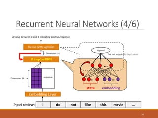
- 35. Recurrent Neural Networks (3/6) Keras offers the SimpleRNN layer to help us construct a simple RNN. In the following example, we sequentially process an IMDB review (i.e., token by token). ◦ Each token is first converted into an embedding (dim. 16). ◦ Then, the SimpleRNN layer processes all the embeddings one by one. ◦ Last, the final output of the RNN layer is fed into a dense layer to predict (classify) the sentiment of the review. 35
- 36. Recurrent Neural Networks (4/6) embeddings … Embedding Layer I do not like this movie … Dimension: 16 SimpleRNN Dense (with sigmoid) Dimension: 16 A value between 0 and 1, indicating positive/negative Input review: … … … state embedding sigmoid The last output of SimpleRNN 36
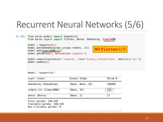
- 37. Recurrent Neural Networks (5/6) NO Flatten()!! 37
- 38. Recurrent Neural Networks (6/6) 38
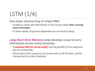
- 39. LSTM (1/4) One major shortcoming of simple RNN: ◦ Unable to retain old information in the current state after running many timesteps. ◦ In other words, long-term dependencies are hard to keep. Long Short-Term Memory (LSTM) develops a way to carry information across many timesteps. ◦ A conveyor belt (or carray track) running parallel to the sequence you are processing. ◦ Information from sequence can jump onto or off the belt, and be transported to a later timestep. 39
- 40. LSTM (2/4) Additional information flow – carry track: ◦ ct the carry at time t. ◦ Connected with the current input and state to affect the state being sent to the next timestep. 40
- 41. LSTM (3/4) Computing the new carry state (i.e., ct+1) is a little bit complicated. ◦ Forget gate, input (candidate) gate, output (update) gate. ◦ We are not going to the detail of these gates. Just keep in mind: the design of LSTM allows past information to be reinjected at a later time. ◦ To have a long term memory of what have happened. 41
- 42. LSTM (4/4) 42