Statistical Distributions
- 1. Data Analysis Course Probability distributions(version-1) Venkat Reddy
- 2. Data Analysis Course • Data analysis design document • Introduction to statistical data analysis • Descriptive statistics • Data exploration, validation & sanitization • Probability distributions examples and Venkat Reddy Data Analysis Course applications • Simple correlation and regression analysis • Multiple liner regression analysis • Logistic regression analysis • Testing of hypothesis • Clustering and decision trees • Time series analysis and forecasting • Credit Risk Model building-1 2 • Credit Risk Model building-2
- 3. Note • This presentation is just class notes. The course notes for Data Analysis Training is by written by me, as an aid for myself. • The best way to treat this is as a high-level summary; the actual session went more in depth and contained other Venkat Reddy Data Analysis Course information. • Most of this material was written as informal notes, not intended for publication • Please send questions/comments/corrections to venkat@trenwiseanalytics.com or 21.venkat@gmail.com • Please check my website for latest version of this document -Venkat Reddy 3
- 4. Contents • What is probability distribution? • Normal distribution • Binomial distribution • Sampling distributions Venkat Reddy Data Analysis Course 4
- 5. Distribution Results of a mathematics test marks from last 10 years School A School B Venkat Reddy Data Analysis Course • Which school is better? • If we are going to conduct another test, how many students can be expected to score 91 to 100 from school A & from school B • This is a frequency distribution of marks. • What is the probability that a student will score more than 50 from school A & from 5 School B?
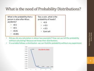
- 6. What is the need of Probability Distributions? What is the probability that a Toss a coin, what is the person is alive after 4 bus probability of heads? accidents? • =0.5 • =0.5 • > 0.5 • >0.5 • < 0.5 • <0.01 • Cant tell Venkat Reddy Data Analysis Course • <0.001 • Did you do any calculation in above two examples? How can we tell the probability without calculating? Because we know their distributions • If a variable follows a distribution we can find the probability without any experiment Accidents data 6
- 7. Roll of a die p(x) x p(x) Probability mass 1 p(x=1)=1/6 function (pmf) 2 p(x=2)=1/6 3 p(x=3)=1/6 1/6 4 p(x=4)=1/6 x 5 p(x=5)=1/6 1 2 3 4 5 6 Venkat Reddy Data Analysis Course 6 p(x=6)=1/6 P(x) 1 all x 1.0 Cumulative distribution x P(x≤A) function (CDF) 1 P(x≤1)=1/6 2 P(x≤2)=2/6 1.0 P(x) 3 P(x≤3)=3/6 5/6 2/3 4 P(x≤4)=4/6 1/2 1/3 5 P(x≤5)=5/6 1/6 6 P(x≤6)=6/6 7 1 2 3 4 5 6 x 0 P( y) 1, P( y) 1
- 8. Probability function f(x)=0.5 for x= ‘Heads’. ‘Tails’ in coin tossing f(x)= 1/6 for x=1,2,3,4,5,6 for roll of dice f(x)=0.2 for x=1,2,3,4,5 or more for accidents example? Venkat Reddy Data Analysis Course Which of the following are probability functions? a. f(x)=.25 for x=9,10,11,12 b. f(x)= (3-x)/2 for x=1,2,3,4 c. f(x)= (x2+x+1)/25 for x=0,1,2,3 8
- 9. Binomial Distribution Data Analysis Course 9 Venkat Reddy
- 10. Binomial Distribution • Suppose we flip a coin 2 times H H HT T H T T • Sample space shows 4 possible outcomes or sequences. Each sequence is a permutation. Order matters. • There are 2 ways to get a total of one heads (HT and TH). These are combinations. Order does NOT matter. HH, HT, TH, Venkat Reddy Data Analysis Course TT • Suppose our interest is Heads. If the coin is fair, p(Heads) = .5; q = 1-p = .5. • The probability of any permutation for 2 trials is ¼ = p*p, or p*q, or q*p, or q*q. All permutations are equally probable. • The probability of 1 head in any order is 2/4 = .5 = 10 HT+TH/(HH+HT+TH+TT)
- 11. Coin example - more flips • 3 flips • HHH, • HHT,HTH,THH • HTT, THT, TTH Venkat Reddy Data Analysis Course • TTT • All permutations equally likely = p*p*p = (1/2)3 = 1/8. • p(0 tail) = 1/8 • p(1 tail) = 3/8 • P(two tails) =?? • P(three tails) =?? 11
- 12. Coin example • 3 flips for count of number of tails • HHH, - Zero out of 3 (3C0?) • HHT,HTH,THH - one out of 3 (3C1?) • HTT, THT, TTH - two out of 3 (3C2?) Venkat Reddy Data Analysis Course • TTT - three out of 3 (3C3?) • All permutations equally likely = p*p*p = .53 = .125 = 1/8. • p(1 tail) = 3/8 =(3c1)(1/2)(1/4) • P(two tails) =(3c1)(1/2)(1/4) • P(three tails) =?? 12
- 13. Binomial Distribution • Black /White choose a color • Out of 4 students , what is the probability that • 0 choose Black & 4 choose White • WWWW - Zero out of 4 (4C0?) • 1 choose Black & 3 choose White Venkat Reddy Data Analysis Course • BWWW, WBWW, WWBW, WWWB - - One out of 4 (4C1?) • 2 choose Black & 2 choose White • 3 choose Black & 1 choose White • 4 choose Black & 0 choose White Which graph best describes the behavior of this count variable? 13
- 14. Binomial distribution function n x P( x) C p q n x x n! C n x!(n x)! x Venkat Reddy Data Analysis Course np npq 2 npq 14
- 15. Binomial distribution -Properties The binomial distribution describes the behavior of a count variable X if the following conditions apply: • The number of observations n is fixed. • Each observation is independent. • Each observation represents one of two outcomes ("success" or "failure"). • The probability of "success" p is the same for each outcome. Venkat Reddy Data Analysis Course 15
- 16. Mean of a distribution • On an average, how many people will chose black? • Like frequency distributions, probability distributions have descriptive measures, such as mean and standard deviation Venkat Reddy Data Analysis Course E (Y ) yP( y) Calculate the mean for color example 16
- 17. Lab • One player stand in the foul line to shoot free-throws 10 times. Suppose the probability that he makes it is 0.5 • Does this meet the criteria of a binomial distribution? • What is the mean and variance? Venkat Reddy Data Analysis Course • What is the probability that he get 6 out of 10? What is the mean and variance? • What is the probability that he get 8 out of 10? • What is the probability that he get 10 out of 10? 17
- 18. Normal distribution Data Analysis Course 18 Venkat Reddy
- 19. Why are normal distributions so important? • The normal distribution is one of the most important distributions in statistics. • Many dependent variables are commonly assumed to be normally distributed in the population • If a variable is approximately normally distributed we can make Venkat Reddy Data Analysis Course inferences about values of that variable • Many measured quantities in the natural sciences follow a normal distribution. • Example: Sampling distribution of the mean 19
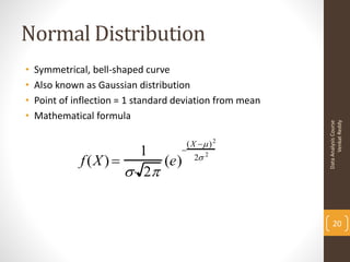
- 20. Normal Distribution • Symmetrical, bell-shaped curve • Also known as Gaussian distribution • Point of inflection = 1 standard deviation from mean • Mathematical formula Venkat Reddy Data Analysis Course (X ) 2 1 f (X ) (e) 2 2 2 20
- 21. Properties of Normal Distribution • The mean, median, and mode are equal • Bell shaped and is symmetric about the mean • The total area that lies under the curve is one or 100% • As the curve extends farther and farther away from the mean, Venkat Reddy Data Analysis Course it gets closer and closer to the x-axis but never touches it. 21
- 22. Empirical Rule About 68% of the area lies within 1 standard deviation of the mean 68% Venkat Reddy Data Analysis Course About 95% of the area lies within 2 standard deviations About 99.7% of the area lies within 3 standard 22 deviations of the mean
- 23. The Standard Normal Distribution • Using the normal probability distribution function, calculate the probity of X >26 when mean is 20 and standard deviation is 6 (X ) 2 1 f (X ) (e) 2 2 2 Venkat Reddy Data Analysis Course • Using the normal probability distribution function, calculate the probity of X >1 when mean is 0 and standard deviation is 1 –Use previous slide • Is it same as Z> (26-20/6) • The standard normal distribution has a mean of 0 and a standard deviation of 1. • Using z-scores any normal distribution can be transformed into the standard normal distribution. 23
- 24. The Standard Score The standard score, or z-score, represents the number of standard deviations a random variable x falls from the mean. Venkat Reddy Data Analysis Course The test scores for a civil service exam are normally distributed with a mean of 152 and a standard deviation of 7. Find the standard z-score for a person with a score of: (a) 161 (b) 148 (c) 152 (a) (b) (c) 24
- 25. Example-1 • The heights of fully grown magnolia bushes have a mean height of 8 feet and a standard deviation of 0.7 feet. 38 bushes are randomly selected from the population, and the mean of each sample is determined. • The mean of the sampling distribution is 8 feet, and the standard error of the sampling distribution is 0.11 feet. • Find the probability that the mean height of the 38 bushes is less than 7.8 Venkat Reddy Data Analysis Course feet. μx = 8 n = 38 σ x = 0.11 x 7.6 8 8.4 25 7.8
- 26. Finding Probabilities Example continued: Find the probability that the mean height of the 38 bushes is less than 7.8 feet. μx = 8 n = 38 σ x = 0.11 x - μx Venkat Reddy Data Analysis Course z P(x < 7.8) σx x 7.8 - 8 7.6 8 8.4 = 7.8 0.11 z 0 = -1.82 P(x < 7.8) = P(z < 1.82) = 0.0344 The probability that the mean height of the 38 bushes is less than 7.8 feet is 0.0344. 26
- 27. Example2 • The average on a statistics test was 78 with a standard deviation of 8. If the test scores are normally distributed, find the probability that the mean score of 25 randomly selected students is between 75 and 79. x - μx 75 - 78 Venkat Reddy Data Analysis Course μx = 78 z1 = = = -1.88 σx 1.6 σ x = σ = 8 = 1.6 n 25 z 2 = x - μ = 79 - 78 = 0.63 P(75 < x < 79) σ 1.6 75 78 79 27 z 1.88 ? 0 0.63 ?
- 28. Finding the probability P(75 < x < 79) Venkat Reddy Data Analysis Course 75 78 79 z 1.88 ? 0 0.63 ? P(75 < x < 79) = P(1.88 < z < 0.63) = P(z < 0.63) P(z < 1.88) = 0.7357 0.0301 = 0.7056 Approximately 70.56% of the 25 students will have a mean score between 75 and 79. 28
- 29. Example 3 x Venkat Reddy Data Analysis Course 3.3 3.6 3.9 4.2 4.5 4.8 5.1 An instruction manual claims that the assembly time for a product is normally distributed with a mean of 4.2 hours and standard deviation 0.3 hour. Determine the interval in which 95% of the assembly times fall. 95% of the data will fall within 2 standard deviations of the mean. 4.2 – 2 (0.3) = 3.6 and 4.2 + 2 (0.3) = 4.8. 29 95% of the assembly times will be between 3.6 and 4.8 hrs.
- 30. Lab • If birth weights in a population are normally distributed with a mean of 3 kg and a standard deviation of 0.3 kg • What is the chance of obtaining a birth weight of 5 kg or heavier when sampling birth records at random? • What is the chance of obtaining a birth weight of 2kg or lighter? Venkat Reddy Data Analysis Course • What is the chance of obtaining a birth weight of 10 kg or heavier? • What is the chance of obtaining a birth weight of 1kg or lighter? • In the instruction manual example(example-3 ) what is the probability that the assembly time is • More than 4 hours? • More than 6 hours? • Less than 3 hours? 30 • Less than 4.2 hours?
- 31. Central Limit Theorem Data Analysis Course 31 Venkat Reddy
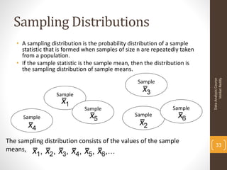
- 32. Sampling Distributions • A sampling distribution is the probability distribution of a sample statistic that is formed when samples of size n are repeatedly taken from a population. Sample7 Venkat Reddy Data Analysis Course Sample2 Sample6 Sample10 Sample1 Sample8 Sample3 Sample5 Sample4 Sample9 32 population
- 33. Sampling Distributions • A sampling distribution is the probability distribution of a sample statistic that is formed when samples of size n are repeatedly taken from a population. • If the sample statistic is the sample mean, then the distribution is the sampling distribution of sample means. Venkat Reddy Data Analysis Course Sample Sample Sample Sample Sample Sample The sampling distribution consists of the values of the sample 33 means,
- 34. Central Limit theorem If a sample n (30) is taken from a population with any type distribution that has a mean = and standard deviation = the sample means will have a normal distribution and standard deviation Venkat Reddy Data Analysis Course 34 x
- 35. Lab • Open excel • Fill column a with random numbers (use ran between function) • In column B, find the mean of first 30 observations from A and Venkat Reddy Data Analysis Course drag it • Draw a histogram of B. 35
- 36. Application Central Limit Theorem • During a certain week the mean price of gasoline in California was $1.164 per gallon. What is the probability that the mean price for the sample of 38 gas stations in California is between $1.169 and $1.179? Assume the standard deviation = $0.049. Venkat Reddy Data Analysis Course mean standard deviation Calculate the standard z-score for sample values of $1.169 and $1.179. 36
- 37. Probabilities of x and x The population mean salary for auto mechanics is $34,000 with a standard deviation of $2,500. Find the probability that the mean salary for a randomly selected sample of 50 mechanics is greater than $35,000. Venkat Reddy Data Analysis Course μx = 34000 x - μx 35000 - 34000 = 2.83 z σ x σ = 2500 = 353.55 = σx 353.55 n 50 P(X> 35000) = P(z > 2.83) = 1 P(z < 2.83) = 1 0.9977 = 0.0023 The probability that the mean salary for a randomly selected sample of 50 34000 35000 37 mechanics is greater than $35,000 is z 0 ? 2.83 0.0023.
- 38. Probabilities of x and x The population mean salary for auto mechanics is = $34,000 with a standard deviation of = $2,500. Find the probability that the salary for one randomly selected mechanic is greater than $35,000. Venkat Reddy Data Analysis Course (Notice that the Central Limit Theorem does not apply.) μ = 34000 z = x - μ = 35000 - 34000 = 0.4 σ 2500 σ = 2500 P(x > 35000) = P(z > 0.4) = 1 P(z < 0.4) = 1 0.6554 = 0.3446 The probability that the salary for 34000 35000 one mechanic is greater than 38 z 0 ? 0.4 $35,000 is 0.3446.
- 39. Looking up probabilities in the standard normal table What is the area to the left of Z=1.51 in a standard normal curve? Venkat Reddy Data Analysis Course Area is 93.45% Z=1.51 39 Z=1.51
- 40. Normal probabilities in SAS data _null_; theArea=probnorm(1.5); The “probnorm(Z)” function gives you the put theArea; probability from negative infinity to Z (here run; 1.5) in a standard normal curve. 0.9331927987 Venkat Reddy Data Analysis Course And if you wanted to go the other direction (i.e., from the area to the Z score (called the so-called “Probit” function data _null_; theZValue=probit(.93); The “probit(p)” function gives you the Z- put theZValue; value that corresponds to a left-tail area of run; p (here .93) from a standard normal curve. 1.4757910282 The probit function is also known as the 40 inverse standard normal function.
- 41. Venkat Reddy Konasani Manager at Trendwise Analytics venkat@TrendwiseAnalytics.com 21.venkat@gmail.com Venkat Reddy Data Analysis Course +91 9886 768879 41


