FEM 10 Common Errors.ppt
The document discusses common errors that can occur in finite element analysis. It identifies two main categories of errors: idealization errors and discretization errors. Idealization errors relate to how the physical problem is simplified, including establishing boundary conditions and material behavior assumptions. Discretization errors occur during the process of replacing the continuous idealized model with a finite element model, and can include issues with imposing boundary conditions, element distortions, and matrix ill-conditioning during the solution process. Overall, the document emphasizes the importance of properly understanding the physical problem, applying appropriate simplifications and boundary conditions, and ensuring a high-quality mesh to minimize errors in finite element analysis.

More Related Content
What's hot
What's hot (20)
Similar to FEM 10 Common Errors.ppt
Similar to FEM 10 Common Errors.ppt (20)
More from Praveen Kumar
More from Praveen Kumar (20)
Recently uploaded
Recently uploaded (20)
FEM 10 Common Errors.ppt
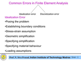
- 1. Common Errors in Finite Element Analysis Idealization error Discretization error Idealization Error •Posing the problem •Establishing boundary conditions •Stress-strain assumption •Geometric simplification •Specifying simplification •Specifying material behaviour •Loading assumptions Prof .N. Siva Prasad, Indian Institute of Technology Madras Error - 1
- 2. Discretization Error •Imposing boundary conditions •Displacement assumption •Poor strain approximation due to element distortion •Feature representation •Numerical integration •Matrix ill-conditioning •Degradation of accuracy during Gaussian elimination •Lack of inter-element displacement compatibility •Slope discontinuity between elements Prof .N. Siva Prasad, Indian Institute of Technology Madras Error - 2
- 3. Idealization Error One must be able to understand the physical nature of an analysis problem well enough to conceive a proper idealization. Engineering assumptions are always required in the process of idealization. Example: •Establishing boundary conditions •Specifying Material behaviour Prof .N. Siva Prasad, Indian Institute of Technology Madras Error - 3
- 4. Establishing Boundary Conditions There are innumerable examples of how the specification of improper boundary conditions can lead to either no results or poor results. It is impractical to review every possible manner in which one can error when establishing boundary conditions. The finite element analyst must gain a sufficient theoretical understanding of mechanical idealization principles so that he can understand what boundary conditions are applicable in any particular case. Consider a bracket loaded by the weight of a servo motor, as illustrated in Figure 1, 2 Prof .N. Siva Prasad, Indian Institute of Technology Madras Error - 4
- 5. Fig 1. Actual Motor Bracket Fig. 2 Simplified Prof .N. Siva Prasad, Indian Institute of Technology Madras Error - 5
- 6. Idealization Error – Specifying Material Behaviour Elasto-Plastic state (Incompressible in plastic region) Elastomeric material (= 0.5, Constitutive relations undefined) Discretization Error Discretization is the process where the idealization, having an infinite number of DOF’s, is replaced with a model having finite number of DOF’s. The following are errors associated with discretization. Prof .N. Siva Prasad, Indian Institute of Technology Madras Error - 6
- 7. No of Points = 8 dof per point = 2 Total Equations = 16 Prof .N. Siva Prasad, Indian Institute of Technology Madras Error - 7
- 8. Element Errors •Imposing essential boundary conditions •Displacement assumption •Poor strain approximation due to element distortion •Feature representation Global Errors •Numerical integration •Matrix ill-conditioning •Degradation of accuracy during Gaussian elimination •Lack of inter-element displacement compatibility •Slope discontinuity between elements Prof .N. Siva Prasad, Indian Institute of Technology Madras Error - 8
- 9. Element Error – Imposing Essential Boundary Conditions Rigid body motion is displacement of a body in such a manner that no strain energy is induced. When one considers finite elements in three-dimensional space, with nodes having three translations DOF’s restraining rigid body motion can be more complicated. Consider the 8-node brick element in three- dimensional space depicted in Figure 4. What are the minimum nodal displacement restraints required to prevent rigid body motion of this element? Prof .N. Siva Prasad, Indian Institute of Technology Madras Error - 9
- 10. Fig 4. 8-node Brick Element in 3-D Space In 3D space, there exists potential for six rigid body modes ( 3 displacements, (x, y, z) and 3 rotations θx, θy and θz ) Prof .N. Siva Prasad, Indian Institute of Technology Madras Error - 10
- 11. Fig 5. Restraining One Node Restraining one node will allow the body to rigidly rotate. Prof .N. Siva Prasad, Indian Institute of Technology Madras Error - 11
- 12. Fig 6. Nodal Restraint as a Ball and Socket Joint Translational motion arrested but the body tend to rotate Prof .N. Siva Prasad, Indian Institute of Technology Madras Error - 12
- 13. Fig 7. Inhibiting Rigid Body Motion Displacement is restrained at 5 and 8. This prevents rotation about z axis. Prof .N. Siva Prasad, Indian Institute of Technology Madras Error - 13
- 14. Most finite element software programs will issue a warning, “singular system encountered” or “Non-positive definite system encountered”. The latter warning refers to the fact that the strain energy is not greater than zero using the given boundary conditions, suggesting that the structure is either unstable, as in the case of structural collapse, or not properly restrained, such that rigid body modes of displacement are possible. Prof .N. Siva Prasad, Indian Institute of Technology Madras Error - 14
- 15. Element Error – Displacement Assumption The h-method of finite element analysis endeavours to minimize this error by using lower order displacement assumptions (typically linear or quadratic) then refining the model using more, smaller elements. Using more smaller elements to gain increased accuracy is known as h- convergence. Prof .N. Siva Prasad, Indian Institute of Technology Madras Error - 15
- 16. Element Error – Poor Strain Approximation Due to Element Distortion Distorted elements influence the accuracy of the finite element approximation for strain. For instance, some bending elements (beams, plated, shells) compute transverse shear stain. This type of elements may have difficulty computing shear strain when the element becomes very thin. Prof .N. Siva Prasad, Indian Institute of Technology Madras Error - 16
- 17. Figure Discretization Error Prof .N. Siva Prasad, Indian Institute of Technology Madras Error - 17
- 18. Global Errors Global errors are those associated with the assembled finite element model. Even if each element exactly represents the displacement within the boundary of a particular element, the assembled model may not represent the displacement within the entire structure, due to global errors. Global Error – Numerical Integration The use of numerical integration instead of closed-form integration introduces error. Prof .N. Siva Prasad, Indian Institute of Technology Madras Error - 18
- 19. Global Error – Matrix Ill-Conditioning The finite elements solution can render poor solutions for displacement due to round off error. Ill-conditioning errors typically manifest themselves during the solution phase of an analysis. Figure: Structure with an Ill-conditioned Stiffness Matrix Prof .N. Siva Prasad, Indian Institute of Technology Madras Error - 19
- 20. A stepped shaft, characterized by two different cross sections, is depicted in Figure. Two rod elements is used to model the structure, with the expanded equilibrium equations for Element I given as: 3 2 1 3 2 1 1 1 1 0 0 0 0 1 1 0 1 1 F F F U U U L A E (1) The equilibrium equations for Elements 2 are: 3 2 1 3 2 1 2 2 2 1 1 0 1 1 0 0 0 0 F F F U U U L A E (2) Prof .N. Siva Prasad, Indian Institute of Technology Madras Error - 20
- 21. Substituting the known variables into the equations above, the stiffness matrices are: 0 0 0 0 0100 . 0 0100 . 0 0 0100 . 0 0100 . 0 0 0 0 1 1 1 0 1 1 00 . 5 ) 0100 . 0 ( 00 . 5 1 K 00 . 1 00 . 1 0 00 . 1 00 . 1 0 0 0 0 1 1 0 1 1 0 0 0 0 00 . 5 ) 00 . 5 ( 00 . 1 2 K (3) (4) Prof .N. Siva Prasad, Indian Institute of Technology Madras Error -21
- 22. The element stiffness matrices are added together to represent the global stiffness: P F U U U 00 . 0 00 . 1 00 . 1 00 . 0 00 . 1 01 . 1 0100 . 00 . 0 0100 . 0100 . 1 3 2 1 (1) Boundary conditions are now imposed upon the global system of Equations, (1). Since U1 = 0 and F1 is unknown, the 3 X 3 system in (1) is replaced by a 2 X 2 systems: P U U 00 . 0 00 . 1 00 . 1 00 . 1 01 . 1 3 2 (2) Prof .N. Siva Prasad, Indian Institute of Technology Madras Error - 22
- 23. Using Gaussian elimination, Equations (2) is manipulated to yield: P U P U U 101 00 . 0 00990 . 00 . 0 00 . 1 01 . 1 3 3 2 (3) Consider a small error in computation of k11 given by Equation(2) P U U 00 . 0 00 . 1 00 . 1 00 . 1 02 . 1 3 2 (4) Prof .N. Siva Prasad, Indian Institute of Technology Madras Error - 23
- 24. Using Gaussian elimination to solve the system containing the small error: 2 3 3 1.02 1.00 0.00 51.0 0.00 .0196 U U P U P (5) It may be surprising to note that a 1% error in one of the entries of the stiffness matrix is responsible for a 50% error in displacement. Prof .N. Siva Prasad, Indian Institute of Technology Madras Error - 24
- 25. 25 EQUILIBRIUM AND COMPATIBILITY IN THE SOLUTION 1.Equilibrium of nodal forces and moments is satisfied. The structural equations {F} – [K] {Q}= {0} are nodal equilibrium equations. Therefore, the solution vector {Q} is such that nodal forces and moments have a zero resultant at every node. 2.Compatibility prevails at nodes. Elements connected to one another have the same displacements at the connection point. (i.e.) elements are compatible at nodes to the extent of nodal d.o.f. they share.
- 26. 26 3. Equilibrium is usually not satisfied across interelement boundaries. Figure 4.4-1 provides a simple example. Imagine that the elements are constant-strain triangles and that node 4 is the only node displaced, as shown. Then σx2 is the only nonzero stress, and the shaded differential element is not in equilibrium
- 27. 27 4. Compatibility may or may not be satisfied across interlement boundaries. The constant-strain triangle and the plane bilinear element, compatibility is guaranteed because element sides remain straight even after the element is deformed. Other elements, such as plate elements are incompatible in rotation about an interlement boundary. Figure 4.4-2 is another case in point. Stretching of the right edge causes vertical edges of the right element to bend, and the interlement gap (shaded) appears. (This element, called either incompatible or nonconforming)
- 28. 28 5.Equilibrium is usually not satisfied within elements. Satisfaction of the differential equations of equilibrium at every point in an element demands a relation among element d.o.f. that usually does not result from solution of the global finite element equations [K]{Q} = {F}. An important property of any reliable element is that its displacement field be capable of representing all possible states of constant strain.
- 29. 29 6. Compatibility is satisfied within elements. We require only that the element displacement field be continuous and single-valued. These properties are automatically provided by polynomial fields. CONVERGENCE REQUIREMENTS 1.Within each element, the assumed field for φ must contain a complete polynomial of degree m. 2.Across boundaries between elements, there must be continuity of φ and its derivatives through order m-1.
- 30. 30 3. Let the elements be used in a mesh (rather than tested individually), and let boundary conditions on the mesh be appropriate to a constant value of any of the mth derivatives of φ. Then, as the mesh is refined, each element must come to display that constant value. For example, if φ = φ(x,y) and П contains first derivatives of φ, then the lowest order acceptable field has the form φ = a1 + a2x + a3y in each element, only φ itself need be continuous across interelement boundaries, and each element of an appropriately loaded mesh must display a constant value of φ,x ( or of φ,y for other appropriate loading), at least as the mesh is refined.
- 31. 31 This suggests the following criterion for modeling. In a mesh of low-order elements (such as the bilinear element), the ratio of stress variation across the element to mean stress within the element should be small. It is a simple test that can be performed numerically, so as to check the validity of an element formulation and its program implementation. We assume that the element is stable in the sense described below. Then, if the element passes the patch test, we have assurance that all convergence criteria are met. THE PATCH TEST
- 32. 32 Procedure. One assembles a small number of elements into a “patch,” taking care to place at least one node within the patch, so that the node is shared by two or more elements, and so that one or more interelement boundaries exist. Figure 4.6-1 shows an acceptable two-dimensional patch, built of four-node elements. Boundary nodes of the patch are loaded by consistently derived nodal loads appropriate to a state of constant stress.
- 33. 33
- 34. 34 Stability. At the outset we assumed that the element to be patch-tested is stable. A stable element is one that admits no zero-energy deformation states when adequately supported against rigid-body motion. Unstable elements should be used with caution. They can produce an unstable mesh, whose displacements are excessive and quite unrepresentative of the actual structure.
- 35. 35 “Weak” Patch Test. An element that fails to display constant stress in a patch of large elements has not necessarily failed the patch test. If, as the mesh is repeatedly subdivided, elements come to display the expected state of constant stress, then the element is said to have passed a “ weak” patch test, and convergence to correct results is assured.
- 36. Convergence To ensure monotonic convergence of the finite element solution, both the individual elements and the assemblage of elements (“the mesh”) must meet certain requirements. Monotonic Convergence Using the Displacement Based, h-Method With mesh refinement, the finite element solution is expected to convergence, monotonically, to the exact solution. Prof .N. Siva Prasad, Indian Institute of Technology Madras Conver - 1
- 37. Prof .N. Siva Prasad, Indian Institute of Technology Madras Conver - 2
- 38. Requirements for Monotonic Convergence (i) Requirements for Each Element’s Displacement Assumption 1. Rigid Body Representation assumption must be able to account for all rigid body displacement modes of the element. 2. Uniform Strain Representation: Constant strain states for all strain components specified in the constitutive equations of a particular idealization must be represented within the element as the largest dimension of the element approaches zero. Prof .N. Siva Prasad, Indian Institute of Technology Madras Conver - 3
- 39. (ii) Requirements for the Mesh 1. Compatibility Between Elements: The dependent variable(s), and p-1 derivatives of the dependent variable, must be continuous at the nodes and across the inter- element boundaries of adjacent elements. 2. Mesh Refinement: Each successive mesh refinement must contain all of the previous nodes and elements in their original location. 3. Uniform Strain Representation: The mesh must be able to represent uniform strain when boundary conditions that are consistent with a uniform strain condition are imposed. Prof .N. Siva Prasad, Indian Institute of Technology Madras Conver - 4
- 40. Understanding Convergence Requirements 1. Convergence and Rigid Body Representation Prof .N. Siva Prasad, Indian Institute of Technology Madras Conver - 5
- 41. In a one-dimensional element with rectangular coordinates, a polynomial displacement assumption must have a constant term to ensure that the type of rigid body motion described above is allowed. U(X) = a1 +a2X 2. Convergence and Uniform Strain Representation within an Element dx du E E xx xx 2 2 1 ) ( a dx du x a a x u xx Prof .N. Siva Prasad, Indian Institute of Technology Madras Conver - 6
- 42. 3. Convergence and Inter-Element Compatibility Continuity must be maintained across element boundaries, as well as at the nodes. A. Incompatibility due to Elements Not Properly Connected: Prof .N. Siva Prasad, Indian Institute of Technology Madras Conver - 7
- 43. Figure shows that Nodes 2 and 3 are coincident nodes, meaning that they have the same spatial coordinated but belong to separate elements. Element Node a Node b 1 1 2 2 3 4 Connectivity table before node merge Prof .N. Siva Prasad, Indian Institute of Technology Madras Conver - 8
- 44. Connectivity table after node merge Element Node a Node b 1 1 2 2 2 3 When creating finite element models, a node merging procedure is typically invoked, such that each pair of coincident nodes is replaced by a single node, and the connectivity table is updated to reflect the new connectivity. Prof .N. Siva Prasad, Indian Institute of Technology Madras Conver - 9
- 45. B. Incompatibility due to Differing Order Displacement Assumptions: Prof .N. Siva Prasad, Indian Institute of Technology Madras Conver - 10
- 46. Consider two elements in Figure 14, one having a linear displacement assumption and other having a quadratic assumption. A gap between the elements occurs since the displacement for the linear element can only be represented by a straight line while displacement in the other element is a quadratic function. Prof .N. Siva Prasad, Indian Institute of Technology Madras Conver - 11
- 47. In figure that the mid-side node of Element 1 is connected to corner nodes of Element 2 and 3. Higher order elements must be matched such that the mid-side node of one element is connected to the mid-side node of the other. Prof .N. Siva Prasad, Indian Institute of Technology Madras Conver - 12
- 48. C. Incompatibility due to Differing Nodal Variables: Prof .N. Siva Prasad, Indian Institute of Technology Madras Conver - 13
- 49. Incompatibility also occurs when element having differing types of nodal DOF are joined. Figure shows a 2-node beam element attached to one node of a 8-node element, which have translational DOF only, while structural elements have both translational and rotational DOF’s. When joining continuum and structural elements, a special constraint must be imposed upon the structural element’s rotational DOF, the least 8-node brick element shown in Figure is well restrained. Its nodes do not have rotational DOF’s, therefore, at the node where the beam is attached, there exits no DOF from the brick to couple with the rotational DOF of the beam. As shown in figure, the beam element will experience rigid body rotation. Prof .N. Siva Prasad, Indian Institute of Technology Madras Conver - 14
- 50. D. Incompatibility due to incompatible elements: Type of incompatibility to be mentioned occurs when elements in mesh are of the “incompatible type” Prof .N. Siva Prasad, Indian Institute of Technology Madras Conver - 15
- 51. Consider the two elements in Figure both are identically formulated, 4 node quadrilateral surface elements designed with incompatible modes of displacement. Assume that two nodes of Element 2 are given a displacement of Δy as depicted in figure (a). With no other displacement, the elements would appear as shown. However, displacement for Element 2 would be computed as shown in figure (18). Prof .N. Siva Prasad, Indian Institute of Technology Madras Conver - 16
- 52. 4. Convergence and the Discretization Process: Each successive mesh refinement must contain all of the previous nodes and elements in their original location. Prof .N. Siva Prasad, Indian Institute of Technology Madras Conver - 17
- 53. 5. Convergence and Uniform Strain Representation within Mesh The mesh must be able to represent a uniform strain state, when suitable boundary conditions are imposed. A Patch Test has been devised to test the uniform strain condition. Either displacements or loads can be applied, depending upon what characteristics of the mesh are to be investigated. Prof .N. Siva Prasad, Indian Institute of Technology Madras Conver - 18
- 54. Figure illustrates a mesh for a patch test of two- dimensional elements although, theoretically, substantial variation in the geometry (somewhat distorted) of the elements used for a patch test is permitted. Prof .N. Siva Prasad, Indian Institute of Technology Madras Conver - 19
- 55. Elementary Beam, Plate, and Shell Elements Euler-Beronoulli Beams Beams are slender structural members, with one dimension significantly greater that the other two. Prof .N. Siva Prasad, Indian Institute of Technology Madras Beam - 1
- 56. Euler-Beronoulli Beam Assumptions If Euler- Bernoulli (“elementary”) beam theory is to be used, some restrictions must be imposed to ensure suitable accuracy. Six items related to the Euler- Beronulli beam bending assumptions are considered in brief: 1. Slenderness (Transverse shear neglected, L/h ≥ 10, Orthogonal planes remain plane and orthogonal) 2. Straight, narrow, and uniform beams (Arch structure – membrane forces.) 3. Small deformations (Second order terms and dropped from the Green-Lagrange Strain mertic) Prof .N. Siva Prasad, Indian Institute of Technology Madras Beam - 2
- 57. 4. Bending loads only (Loads that cause twist or cause x- or y- displacement of neutral axis are ignored.) 5. Linear, isotropic, homogeneous materials response 6. Only normal stress in the x-coordinate direction (σxx) significant (σxx vary linearly in the z direction and σzz = 0 Prof .N. Siva Prasad, Indian Institute of Technology Madras Beam - 3
- 58. Kirchhoff Plate Bending Assumptions Several restrictions must be imposed when using the Kirchhoff plate bending formulation if suitable accuracy is to be obtained; six related items are considered briefly: 1. Thinness 2. Flatness and uniformity 3. Small deformation 4. No membrane deformation 5. Linear, isotropic, homogeneous materials 6. σxx, σyy , σxy the only stress components of significance Prof .N. Siva Prasad, Indian Institute of Technology Madras Beam - 4
- 59. 1.Thin Plates: If the ratio of the in-plane dimensions to thickness is greater than ten, a plate may be considered thin; in other words, thin plates are such that . 10 / / t b t l (i) Transverse Shear Stress Does Not Affect Transverse Displacement: Although transverse displacement of a plat loaded normal to its neutral surface is affected by both normal stress and transverse shear stress, it is assumed that the shear stress does not have a significant impact on the magnitude of transverse displacement. It can be shown that the magnitude of transverse displacement due to shear stress is small in thin plates. Prof .N. Siva Prasad, Indian Institute of Technology Madras Beam - 5
- 60. (ii) Orthogonal Planes Remain Plane and Orthogonal: In a thin plate, any cross sectional plane, originally orthogonal to the neutral surface, is assumed to remain plane and orthogonal when the plate is loaded. As with deep beams, cross sections in thick plates, originally orthogonal and planar, will be neither under transverse load, due to shearing effects. Prof .N. Siva Prasad, Indian Institute of Technology Madras Beam - 6
- 61. 2. Flat and Uniform Kirchhoff plates are presumed flat, and as such, loads are not carried by membrane deformation. If initial curvature were to exist, some of the load could be carried by membrane action, hence, curved plates (shells) require a different approach to account for the combination of simultaneous membrane and bending deformation. Prof .N. Siva Prasad, Indian Institute of Technology Madras Beam - 7
- 62. 3. Small Deformation 1. The expression for stain actually contains second order terms, and these terms are truncated if the strains are presumed small. 2. Like the Euler-Bernoulli beam, plate curvature can be expressed in terms of second order derivatives if the square of the slop is negligible. 3. As a plate deflects its transverse stiffness changes. Prof .N. Siva Prasad, Indian Institute of Technology Madras Beam - 8
- 63. Why does the transverse stiffness change with deflection? As a plate deforms into a curved (or a doubly curved) surface, transverse loads are resisted by both bending and membrane deformation. The addition of membrane deformation affects the transverse stiffness of the plate. Consider figure where a ball is placed on a very thin “plate”. Notice that as the amount of plate deflection increases, more load is carried by membrane tension and less by bending. Shell theory is required to account for structure that carry loads through simultaneous bending and membrane deformation Prof .N. Siva Prasad, Indian Institute of Technology Madras Beam - 9
- 64. 4. No Membrane Deformation Kirchhoff plates do not account for membrane deformation. This means that at the neutral surface, there can be no displacement in the x- or y-coordinate directions, which would suggest the existence of membrane deformation 5. Signification Stress Components are σ xx, σ yy , σ xy As in shallow beams, it is assumed that transverse shear stress in thin plates is relatively insignificant when compared to the normal stress in the longitudinal direction of the beam, hence: σyz = σzx = 0 and σzz = 0 Prof .N. Siva Prasad, Indian Institute of Technology Madras Beam - 10
- 65. Shear Stress Affects the Edge Reaction Forces In plate bending stress affects transverse displacement. In addition, shear stress affects reaction forces on restrained edges of plates and shells. The restrained edges of shell and plate structures develop reaction forces. The magnitude of the reaction is dependent upon the behaviour in the vicinity very near the restrained edge. This boundary layer effect cannot be captured without accounting for transverse shear stress. In addition, even in models that do account for shear effects, the boundary layer effect is difficult to model without special care. Prof .N. Siva Prasad, Indian Institute of Technology Madras Beam - 11