


Fm ppt unit 5
- 1. Fluid Mechanics Prepared By: Md Ateeque Khan Assistant Professor JIT 5/26/2017 JIT 1
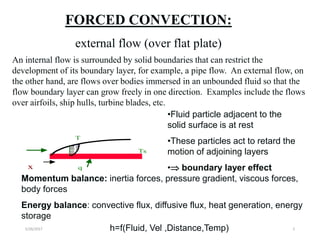
- 2. les x q Ts T h=f(Fluid, Vel ,Distance,Temp) •Fluid particle adjacent to the solid surface is at rest •These particles act to retard the motion of adjoining layers • boundary layer effect Momentum balance: inertia forces, pressure gradient, viscous forces, body forces Energy balance: convective flux, diffusive flux, heat generation, energy storage FORCED CONVECTION: external flow (over flat plate) An internal flow is surrounded by solid boundaries that can restrict the development of its boundary layer, for example, a pipe flow. An external flow, on the other hand, are flows over bodies immersed in an unbounded fluid so that the flow boundary layer can grow freely in one direction. Examples include the flows over airfoils, ship hulls, turbine blades, etc. 5/26/2017 JIT 2
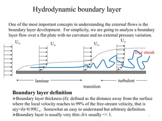
- 3. One of the most important concepts in understanding the external flows is the boundary layer development. For simplicity, we are going to analyze a boundary layer flow over a flat plate with no curvature and no external pressure variation. laminar turbulent transition Dye streak U U U U Hydrodynamic boundary layer Boundary layer definition Boundary layer thickness (d): defined as the distance away from the surface where the local velocity reaches to 99% of the free-stream velocity, that is u(y=d)=0.99U. Somewhat an easy to understand but arbitrary definition. Boundary layer is usually very thin: d/x usually << 1.5/26/2017 JIT 3
- 4. Hydrodynamic and Thermal boundary layers • As we have seen earlier,the hydrodynamic boundary layer is a region of a fluid flow, near a solid surface, where the flow patterns are directly influenced by viscous drag from the surface wall. • 0<u<U, 0<y<d • The Thermal Boundary Layer is a region of a fluid flow, near a solid surface, where the fluid temperatures are directly influenced by heating or cooling from the surface wall. • 0<t<T, 0<y<dt • The two boundary layers may be expected to have similar characteristics but do not normally coincide. Liquid metals tend to conduct heat from the wall easily and temperature changes are observed well outside the dynamic boundary layer. Other materials tend to show velocity changes well outside the thermal layer.5/26/2017 JIT 4
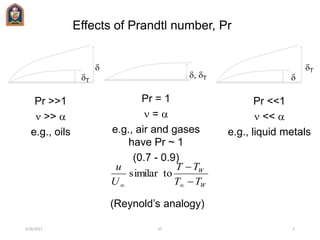
- 5. Effects of Prandtl number, Pr d dT Pr >>1 >> e.g., oils d, dT Pr = 1 = e.g., air and gases have Pr ~ 1 (0.7 - 0.9) W W TT TT U u tosimilar (Reynold’s analogy) dT d Pr <<1 << e.g., liquid metals 5/26/2017 JIT 5
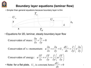
- 6. Boundary layer equations (laminar flow) • Simpler than general equations because boundary layer is thin d dT U WT T U x y • Equations for 2D, laminar, steady boundary layer flow y T yy T v x T u y u ydx dU U y u v x u u y v x u :energyofonConservati :momentum-xofonConservati 0:massofonConservati • Note: for a flat plate, 0hence,constantis dx dU U5/26/2017 JIT 6
- 7. Exact solutions: Blasius 3 1 2 1 3 1 2 1 PrRe678.0numberNusseltAverage PrRe339.0numberNusseltLocal Re Re 328.11 tcoefficiendragAverage ,Re Re 664.0 tcoefficienfrictionSkin Re 99.4 x knesslayer thicBoundary 0 0 2 2 1 L xx L L L fD y wx x w f x uN Nu LU dxC L C y uxU U C d 5/26/2017 JIT 7
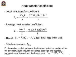
- 8. Heat transfer coefficient • Local heat transfer coefficient: x k x kNu h xx x 3 1 2 1 PrRe339.0 • Average heat transfer coefficient: L k L kuN h L 3 1 2 1 PrRe678.0 • Recall: wallfromrateflowheat, TTAhq ww• Recall: wallfromrateflowheat, TTAhq ww • Film temperature, Tfilm For heated or cooled surfaces, the thermophysical properties within the boundary layer should be selected based on the average temperature of the wall and the free stream; TTT wfilm 2 1 5/26/2017 JIT 8
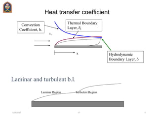
- 9. Heat transfer coefficient U x Hydrodynamic Boundary Layer, d Convection Coefficient, h. Thermal Boundary Layer, dt Laminar Region Turbulent Region Laminar and turbulent b.l. 5/26/2017 JIT 9
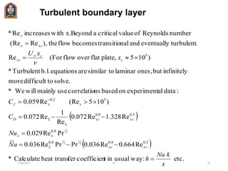
- 10. Turbulent boundary layer etc.:wayusualintcoefficienferheat transCalculate* Re664.0Re036.0PrPrRe036.0 PrRe029.0 Re328.1Re072.0 Re 1 Re072.0 )105(ReRe059.0 :dataalexperimentonbasednscorrelatiousemainlywillWe* solve.todifficultmore infinitelybutones,laminarsimilar toareequationsb.l.Turbulent* )105plate,flatoverflowFor(Re .turbulenteventuallyandnaltransitiobecomesflowthe),ReRe( numberReynoldsofvaluecriticalaBeyondwith x.increasesRe* 5.08.08.0 8.0 5.08.0 52.0 5 3 1 3 1 3 1 x kNu h uN Nu C C x xU xcxcL xx xcxc L LD xxf c c xc xcx x 5/26/2017 JIT 10
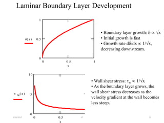
- 11. d x( ) x 0 0.5 1 0 0.5 1 • Boundary layer growth: d x • Initial growth is fast • Growth rate dd/dx 1/x, decreasing downstream. w x( ) x 0 0.5 1 0 5 10 • Wall shear stress: w 1/x • As the boundary layer grows, the wall shear stress decreases as the velocity gradient at the wall becomes less steep. Laminar Boundary Layer Development 5/26/2017 JIT 11
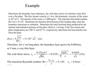
- 12. Determine the boundary layer thickness, the wall shear stress of a laminar water flow over a flat plate. The free stream velocity is 1 m/s, the kinematic viscosity of the water is 10-6 m2/s. The density of the water is 1,000 kg/m3. The transition Reynolds number Re=Ux/=5105. Determine the distance downstream of the leading edge when the boundary transitions to turbulent. Determine the total frictional drag produced by the laminar and turbulent portions of the plate which is 1 m long. If the free stream and plate temperatures are 100 C and 25 C, respectively, determine the heat transfer rate from the plate. 3 2 w ( ) 5 5 10 ( ). Therefore, for a 1m long plate, the boundary layer grows by 0.005(m), or 5 mm, a very thin layer. 0.332 0.0105 The wall shear stress, 0.332 ( ) Re The transition Reyn x x x x m U U U U Pa x x d 5U olds number: Re 5 10 , 0.5( )tr tr x x m Example 5/26/2017 JIT 12
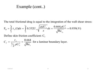
- 13. 2 D 0 0 f 2 The total frictional drag is equal to the integration of the wall shear stress: 0.664 F (1) 0.332 0.939( ) Re Define skin friction coefficient: C 0.664 for a 1 Re 2 tr tr tr x x w x w f x U U dx U dx N x C U laminar boundary layer. Example (cont..) 5/26/2017 JIT 13
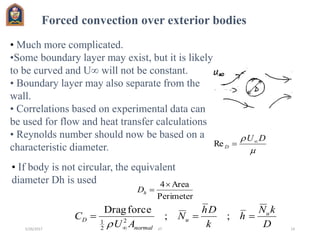
- 14. DU D Re Perimeter Area4 hD D kN h k Dh N AU C u u normal D ;; forceDrag 2 2 1 Forced convection over exterior bodies • Much more complicated. •Some boundary layer may exist, but it is likely to be curved and U will not be constant. • Boundary layer may also separate from the wall. • Correlations based on experimental data can be used for flow and heat transfer calculations • Reynolds number should now be based on a characteristic diameter. • If body is not circular, the equivalent diameter Dh is used 5/26/2017 JIT 14
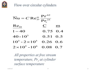
- 15. 0.70.0810-102 0.60.26102-10 0.50.5110-40 0.40.75401 mCRe Pr Pr ReuN 65 53 3 D 25. 62. s m DC Flow over circular cylinders All properties at free stream temperature, Prs at cylinder surface temperature 5/26/2017 JIT 15
- 16. • Thermal conditions Laminar or turbulent entrance flow and fully developed thermal condition For laminar flows the thermal entrance length is a function of the Reynolds number and the Prandtl number: xfd,t/D 0.05ReDPr, where the Prandtl number is defined as Pr = / and is the thermal diffusitivity. For turbulent flow, xfd,t 10D. FORCED CONVECTION: Internal flow Thermal entrance region, xfd,t e.g. pipe flow 5/26/2017 JIT 16
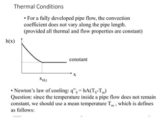
- 17. Thermal Conditions 5/26/2017 JIT 17 • For a fully developed pipe flow, the convection coefficient does not vary along the pipe length. (provided all thermal and flow properties are constant) x h(x) xfd,t constant • Newton’s law of cooling: q”S = hA(TS-Tm) Question: since the temperature inside a pipe flow does not remain constant, we should use a mean temperature Tm , which is defines as follows:
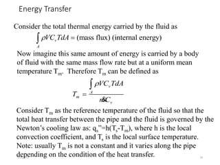
- 18. Energy Transfer 5/26/2017 JIT 18 Consider the total thermal energy carried by the fluid as (mass flux) (internal energy)v A VC TdA Now imagine this same amount of energy is carried by a body of fluid with the same mass flow rate but at a uniform mean temperature Tm. Therefore Tm can be defined as v A m v VC TdA T mC & Consider Tm as the reference temperature of the fluid so that the total heat transfer between the pipe and the fluid is governed by the Newton’s cooling law as: qs”=h(Ts-Tm), where h is the local convection coefficient, and Ts is the local surface temperature. Note: usually Tm is not a constant and it varies along the pipe depending on the condition of the heat transfer.
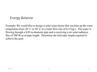
- 19. Energy Balance 5/26/2017 JIT 19 Example: We would like to design a solar water heater that can heat up the water temperature from 20° C to 50° C at a water flow rate of 0.15 kg/s. The water is flowing through a 0.05 m diameter pipe and is receiving a net solar radiation flux of 200 W/m of pipe length. Determine the total pipe length required to achieve the goal.
- 20. 5/26/2017 JIT 20