


Geographic information system(GIS) and its applications in agriculture
- 1. Presented by, Nalla Anthony Kiranmai 15PAGR04 AGR 591 SEMINAR (0+1) CHAIRMAN: Dr. R. MOHAN Professor, Dept. of Agronomy MEMBERS: Dr. R. POONGUZHALAN Professor and Head, Dept. of Agronomy Dr. S. NADARADJAN Asst. Prof. (Crop physiology) Dept. of Plant breeding and genetics.
- 2. Topics of discussion • Introduction • Principle of Geographic information system – Definition • Components of GIS • Information storage • Spatial data representation • Vector Vs Raster • Spatial objects • GIS functions • Linkage between Remote sensing and GIS • Remote sensing supported GIS operations • Conceptual Model of GIS • GIS – An Integrating Technology • How a GIS holds data • Map Scale • Creating a GIS • Data sources
- 3. • Building a GIS • Advantages and Disadvantage of GIS • Fields where GIS is applicable • Weather, Soil and Agriculture applications of GIS • GIS Applications • GIS in Land suitability studies • Integrated Assessment of Groundwater for Agricultural Use • Study on spatial variability of PAJANCOA East farm soils using GIS • GIS in yield forecasting • GIS in drought assessment • Advantages and disadvantages • Conclusion Contd.,
- 4. GIS = G + IS = Geographic reference + Information system Spatial coordinates on the surface of the earth Database All data in GIS must be linked to a geographic reference Introduction
- 5. It is an organized collection of computer hardware , software, geographic data and the personnel designed to efficiently capture, store, retrieve, update, manipulate, analyze and display all forms of geographically referenced information according to the user defined specifications. Principle of Geographic information system Definition
- 6. Tool for handling geographic data. Geographic Information System Spatial data Descriptive data Location, shape and relationship among the features Characteristics of the features.
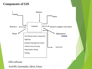
- 7. Components of GIS GIS software ArcGIS, Geomedia, Idrisi, Grass
- 8. Information storage Spatial data Attribute data: Eg. Well locations or sampling points River and road networks Fields, soil delineations, or land use classes. Points, lines, polygons. Eg. Characteristics of the spatial feature Soil map unit - predominant soil series, soil drainage class, and texture of the surface soil horizon Color, symbol, patterns.
- 9. Spatial data Attribute data
- 10. Spatial data representation: Represented by points , lines, polygons Ability to visualize the geographic data by linking the geographic data to the visual data elements (point, line, areas) which compose the picture. Visual data Raster vector
- 11. Raster • Raster data represent a point, a line or an area as a matrix of values. • The size of the cell determines the resolution of the display. • A raster database requires that all the values or entities be defined by a single raster or group of raster
- 12. Vector Points are usually represented by Cartesian coordinates(x, y), a line by a string of coordinates and an area or polygon by a string of coordinates starting and ending at the same point. A vector model defines graphic elements using basic geometry, namely a quantity which has magnitude and direction, represented by a directed line the length representing the magnitude and whose orientation in space represent the direction.
- 13. Vector Vs Raster Fig source: http://www.extension.umn.edu
- 14. 14 Vector and Raster Formats RASTER VECTOR
- 15. 15 Most GIS software permit Raster-Vector format conversions: Fig Source: FAO Vector to raster - easy Raster to vector - hard
- 16. Spatial objects:
- 17. GIS functions Data input functions: Existing form Form that is suitable for use in the GIS converts Data management functions: • Storage and retrieval of data from the GIS database • Capability to read the data in a flexible and logical manner, to search and identify specific items or attributes, and to display these information in a spatial context.
- 18. Data manipulation and Analysis functions Original spatial data sets geometry Better manageable, accurate and consistent with the other data sets already present or to be encoded in the system Manipulation of spatial data Map overlays Creates new map layers with an existing one Features of each coverage are intersected to create new output features Transform
- 19. 19 Map Layer Overlay Overlay generates homogenous units – eg. agroecozones All layers must be in same projection and scale Fig Source: FAO
- 20. Map dissolve • Deletes the boundaries between adjacent polygons having the same attributes values for a specified feature. • Clipping the unwanted polygons from the map. Buffers Polygons created around points, lines and polygons.
- 21. 21 Buffering Buffering: forming bands on either side of lines or around of points or polygons to perform analysis within the bands
- 22. Data output functions: • The outputs (reports) may be in the form of CRT display, maps, listings, data files or text in hard copy. • CRT display during interactive data processing and map development is an important operational requirement
- 24. Linkage between Remote sensing and GIS • Noninvasive and nondestructive gathering of information • Valuable source of input for GIS databases • Quick collecting of data (often in a digital format) over large areas.
- 25. Remote sensing supported GIS operations • Display backdrop: Visual aid or for the interactive creation and updating of maps. Desired base is a photograph, then scanning is needed to convert it to digital form. • For the generation of thematic maps: Utilized as a data layer for GIS functions. • For the derivation of input variables for models. • Real-time link
- 26. What a GIS can do: Location :What exists at a particular location ? Conditions : Where do certain conditions apply ? Trends : What changes have occurred over time ? Spatial Patterns :What spatial patterns exist ? What if …: What will be the consequences of decisions (GIS + Models)-Spatial Decision Support Systems.
- 27. Conceptual Model of GIS GIS “themes,” “layers,” or “coverages” The real world
- 28. GIS – An Integrating Technology Fig Source: FAO
- 29. How a GIS holds data • GIS holds spatial information in independent map layers – single phenomenon mapped across space • Integrates layers by registering them to a common locational reference (lat/long grid). • Thematic layers can all be made visible at the same time or selectively and linked by common location • Allows overlaying to get homogenous land units and other types of information • Allows collating data from several layers for any location • Allows spatial analysis
- 30. New data can also be entered into a GIS in many different ways, including: – Digitizing from a digitizer – GPS – Surveys, via COGO (computer geometry operations) – Scanned images and Digitization – Acquisition from remote sensing instrumentation
- 31. Map Scale Scale: Ratio of distances on map to distances on earth’s surface Representation: Graphical: km Verbal: 1 cm = 2.5 km Numeric: 1:250000 Preferred representation: graphical
- 32. Map scale determines the size and shape of features • Large scale • Small scale city 1:500 1:24000 1:24000 city 1:250000 Source: ESRI
- 33. Standard Scales: 1:1000,000 Country level 1: 250,000 State level 1: 50,000 District level 1: 12,500 Micro level Survey of India Maps (topographic maps) are available at all scales except 1:12,500
- 34. 34 Creating a GIS Data Input Getting spatial data into GIS Getting attribute data into GIS Data Storage Making data usable Data analysis Geographic analysis Data Output Presenting results
- 35. 35 Fig Source: (Murai and Murai, 1999)) Spatial data Attribute data Data sources
- 36. 36 Building a GIS Data base design Area boundaries Co-ordinate system (datum/projection/GCPs) data layers features for each layer attributes for each feature type coding and organizing attribute data (external database design) Entering spatial data from maps for each layer (digitizing layers) Entering attribute data Managing the data base Presenting maps in customized form
- 37. Fields where GIS is applicable Astronomy/Planetary Disaster management Healthy Mapping Agriculture Ecology Mining Archaeology Economics Ocean / Marine Architecture Energy Politics/Government Aquatics Engineering Soils Aviation Environment Sports & Recreation Automobile Integration Education Surveying Banking Forestry Telecommunications Business & Commerce Geostatistics Tourism Consumer Science and Behavior Groundwater Transmission Planning and Routing Climate Change Geology Utilities Crime Hydrology Volunteer GIS and Open Technology Defense/Military Municipality/Urban Weather
- 38. Weather, Soil and Agriculture applications of GIS: Weather Soil Agriculture Rainfall Soil Types Precision Farming Weather Stations Soil Grid Disease Control Doppler Radar Texture Classification Crop Assimilation Model Cirrus Clouds Soil Moisture Water Stress Weather Warnings Soil Survey Geographic Database Crop Resilience to Climate Change Ocean Surface Current Analysis Real-Time (OSCAR) Water Retention Capacity Crop Productivity Real-time Lightning Erosion Reduction Strategy Irrigation Global Wind Vectors Slope Parameters Drought Albedo Soil Loss Equation Crop Forecasting Solar Irradiance Salinity Organic Farming Snowfall Vegetation Erosion Drainage Ditches 3D Atmospheric Data Normalized Difference Soil Index (NDSI) Length of Growing Period
- 39. 39 GIS Applications Resource Inventory (Data Base Management) Integration of Different Layers (Overlay) Interfacing with simulation models – GIS based DSS Level-1 Level-2 Level-3
- 40. APPLICATIONS OF GIS IN AGRICULTURE
- 41. Ronald and Moses, 2016 Land suitability study for rice growing in Kisumu county(Ronald and Moses,2016)
- 42. Criteria relationship: Ronald and Moses, 2016
- 43. Different parameters considered: Land cover map Interpolated rainfall map
- 44. Interpolated temperature map Slope map Contd.,
- 45. Contd., Soil depth map Soil drainage map
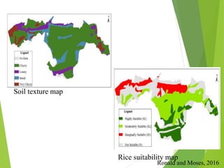
- 46. Soil texture map Rice suitability map Ronald and Moses, 2016
- 47. Rice crop suitability classes in Kisumu county Ronald and Moses, 2016
- 48. Integrated Assessment of Groundwater for Agricultural Use in Mewat District of Haryana, India Using Geographical Information System (GIS) Mamta et al., 2016
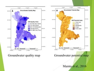
- 49. Groundwater quality map Groundwater potential map Mamta et al., 2016
- 50. Groundwater vulnerability map Integrated groundwater assessment map Mamta et al., 2016
- 51. Characteristics of integrated groundwater map Mamta et al., 2016
- 52. Study on spatial variability of PAJANCOA east farm soils using GIS: East Farm map of PAJANCOA & RI, Karaikal with sampling points Aruna et al., 2016
- 53. • Parameters considered for the study: • pH and EC, • organic carbon, • Available Nitrogen • Available Phosphorus • Available Potassium
- 54. Soil pH variability in east farm of PAJANCOA and RI, Karaikal. Aruna et al., 2016
- 55. Electrical conductivity variability in East farm soils of PAJANCOA & RI, Karaikal Aruna et al., 2016
- 56. Organic carbon variability Aruna et al., 2016
- 57. Aruna et al., 2016 Available Nitrogen variability
- 58. Available Phosphorus variability Aruna et al., 2016
- 59. Available Potassium variability Aruna et al., 2016
- 60. Remote Sensing and GIS Based Spectro-Agrometeorological Maize Yield Forecast Model for South Tigray Zone, Ethiopia Abiy et al., 2016
- 61. • Normalized Difference Vegetation Index • Rainfall Estimate • Water Requirement Satisfaction Index WRSI = (ETa /WR) x 100 ETa = Seasonal actual evapotranspiration WR = Seasonal crop water requirement Where., WR= PET x Kc PET = potential evapotranspiration Kc = crop coefficient Where.,
- 62. Correlation between NDVI Variables and Maize Yield: Maize yield as a function of NDVIa Maize yield as a function of NDVIc NDVIa = actual NDVI NDVIc = cumulative NDVI
- 63. Maize yield as a function of NDVIx Correlation between RFE and Maize Yield Maize yield as a function of RFE
- 64. Correlation between WRSI and Maize Yield: Maize yield as a function of WRSI
- 65. Correlation between ETa Variables and Maize Yield: Maize yield as a function of Eta Maize yield as a function of Eta total.
- 66. Multiple Linear Regression Model for Yield Forecasting: This multiple regression generated the following equation. Predicted Maize Yield (q ha-1) = -1.06 + (21.99 x NDVIa) + (0.24 x REF) Actual yield from spectro-agrometerological model as a function of predicted yield.
- 67. ANOVA of maize yield forecast model. Parameters estimates of the maize forecast model. Abiy et al., 2016
- 68. Evaluation of Conventional Crop Yield Forecast Using the Developed Model: Evaluation of conventional crop yield (q.ha-1) forecast using developed model. Abiy et al., 2016
- 69. Maize yield forecast map of South Tigary zone in Ethiopia for the year 2013. Abiy et al., 2016
- 70. Drought Assessment Using GIS and Remote Sensing in Amman-Zarqa Basin, Jordan Rainfall data satellite images Standardized Precipitation Index (SPI) Normalized Difference Vegetation Index (NDVI • Spatial digital database • Generate thematic layers • Delineate areas with high drought risk • Compare the results of both models GIS software
- 71. Normal Difference Vegetation Index (NDVI) (Tucker, 1979) NDVI = (λNIR - λRED) / (λNIR + λRED) where, λNIR = Reflectance in the near infrared (NIR) λRED = Reflectance in the Red bands It varies in the range of -1 to + 1. DEVNDVI = NDVIi- NDVImean, m Where, DEVNDVI = NDVI deviation NDVIi = NDVI value for month i NDVImean,m = long-term mean NDVI for the same month, m
- 72. NDVI drought Index Map for selected years and selected months. Nezar Hammouri and Ali El-Naqa, 2007
- 73. Standardized Precipitation Index (McKee et al., 1993) Quantify the precipitation scarcity for multiple time scales Long-term record is fitted to a probability distribution, which is transformed into a normal distribution where the mean SPI for the location and desired time period is zero. Classification of SPI Values. (McKee et al., 1993)
- 74. The SPI values for 6 and 12 months for selected stations. (McKee et al., 1993)
- 75. The SPI values for 6 and 12 months for selected stations. (McKee et al., 1993)
- 76. Advantages and Disadvantage of GIS Advantages: Data are stored in a physically compact format and can be retrieved quickly. Spatial analysis is conducted by computer algorithms that, from a practical perspective, are not performed on analog map data, such as multi parameter spatial modeling and change analysis. Spatial and attribute data are integrated into a single system. It is cost effective for certain complex spatial modeling tasks. Data collection, spatial analysis, and decision making are integrated into a single system.
- 77. Disadvantages The cost can be prohibitively high to convert existing maps and attribute. Purchase and maintenance costs of computer software and hardware are high for complex modeling tasks or sustaining large databases. A relatively high level of technical expertise is required for successful GIS. The primary cost when establishing a working GIS involves database development; this accounts for over 90% of the total system cost in some cases. After a digital database is established, however, it can be easily updated and used for numerous applications.
- 78. Conclusion: The agronomic community, including farmers, land managers, fellow scientists, policymakers, and the general public should benefit from this evolving and expanding field.