


HBase in Practice
- 1. HBase in Practice Lars George – Partner and Co-Founder @ OpenCore DataWorks Summit 2017 - Munich NoSQL is no SQL is SQL?
- 2. About Me • Partner & Co-Founder at OpenCore • Before that • Lars: EMEA Chief Architect at Cloudera (5+ years) • Hadoop since 2007 • Apache Committer & Apache Member • HBase (also in PMC) • Lars: O’Reilly Author: HBase – The Definitive Guide • Contact • lars.george@opencore.com • @larsgeorge Website: www.opencore.com
- 3. Agenda • Brief Intro To Core Concepts • Access Options • Data Modelling • Performance Tuning • Use-Cases • Summary
- 4. Introduction To Core Concepts
- 5. HBase Tables • From user perspective, HBase is similar to a database, or spreadsheet • There are rows and columns, storing values • By default asking for a specific row/column combination returns the current value (that is, that last value stored there)
- 6. HBase Tables • HBase can have a different schema per row • Could be called schema-less • Primary access by the user given row key and column name • Sorting of rows and columns by their key (aka names)
- 7. HBase Tables • Each row/column coordinate is tagged with a version number, allowing multi-versioned values • Version is usually the current time (as epoch) • API lets user ask for versions (specific, by count, or by ranges) • Up to 2B versions
- 8. HBase Tables • Table data is cut into pieces to distribute over cluster • Regions split table into shards at size boundaries • Families split within regions to group sets of columns together • At least one of each is needed
- 9. Scalability – Regions as Shards • A region is served by exactly one region server • Every region server serves many regions • Table data is spread over servers • Distribution of I/O • Assignment is based on configurable logic • Balancing cluster load • Clients talk directly to region servers
- 10. Column Family-Oriented • Group multiple columns into physically separated locations • Apply different properties to each family • TTL, compression, versions, … • Useful to separate distinct data sets that are related • Also useful to separate larger blob from meta data
- 11. Data Management • What is available is tracked in three locations • System catalog table hbase:meta • Files in HDFS directories • Open region instances on servers • System aligns these locations • Sometimes (very rarely) a repair may be needed using HBase Fsck • Redundant information is useful to repair corrupt tables
- 12. HBase really is…. • A distributed Hash Map • Imagine a complex, concatenated key including the user given row key and column name, the timestamp (version) • Complex key points to actual value, that is, the cell
- 13. Fold, Store, and Shift • Logical rows in tables are really stored as flat key-value pairs • Each carries full coordinates • Pertinent information can be freely placed in cell to improve lookup • HBase is a column-family grouped key-value store
- 14. HFile Format Information • All data is stored in a custom (open-source) format, called HFile • Data is stored in blocks (64KB default) • Trade-off between lookups and I/O throughput • Compression, encoding applied _after_ limit check • Index, filter and meta data is stored in separate blocks • Fixed trailer allows traversal of file structure • Newer versions introduce multilayered index and filter structures • Only load master index and load partial index blocks on demand • Reading data requires deserialization of block into cells • Kind of Amdahl’s Law applies
- 15. HBase Architecture • One Master and many Worker servers • Clients mostly communicate with workers • Workers store actual data • Memstore for accruing • HFile for persistence • WAL for fail-safety • Data provided as regions • HDFS is backing store • But could be another
- 17. HBase Architecture (cont.) • Based on Log-Structured Merge-Trees (LSM-Trees) • Inserts are done in write-ahead log first • Data is stored in memory and flushed to disk on regular intervals or based on size • Small flushes are merged in the background to keep number of files small • Reads read memory stores first and then disk based files second • Deletes are handled with “tombstone” markers • Atomicity on row level no matter how many columns • Keeps locking model easy
- 18. Merge Reads • Read Memstore & StoreFiles using separate scanners • Merge matching cells into single row “view” • Delete’s mask existing data • Bloom filters help skip StoreFiles • Reads may have to span many files
- 19. APIs and Access Options
- 20. HBase Clients • Native Java Client/API • Non-Java Clients • REST server • Thrift server • Jython, Groovy DSL • Spark • TableInputFormat/TableOutputFormat for MapReduce • HBase as MapReduce source and/or target • Also available for table snapshots • HBase Shell • JRuby shell adding get, put, scan etc. and admin calls • Phoenix, Impala, Hive, …
- 21. Java API From Wikipedia: • CRUD: “In computer programming, create, read, update, and delete are the four basic functions of persistent storage.” • Other variations of CRUD include • BREAD (Browse, Read, Edit, Add, Delete) • MADS (Modify, Add, Delete, Show) • DAVE (Delete, Add, View, Edit) • CRAP (Create, Retrieve, Alter, Purge) Wait what?
- 22. Java API (cont.) • CRUD • put: Create and update a row (CU) • get: Retrieve an entire, or partial row (R) • delete: Delete a cell, column, columns, or row (D) • CRUD+SI • scan: Scan any number of rows (S) • increment: Increment a column value (I) • CRUD+SI+CAS • Atomic compare-and-swap (CAS) • Combined get, check, and put operation • Helps to overcome lack of full transactions
- 23. Java API (cont.) • Batch Operations • Support Get, Put, and Delete • Reduce network round-trips • If possible, batch operation to the server to gain better overall throughput • Filters • Can be used with Get and Scan operations • Server side hinting • Reduce data transferred to client • Filters are no guarantee for fast scans • Still full table scan in worst-case scenario • Might have to implement your own • Filters can hint next row key
- 24. Data Modeling Where’s your data at?
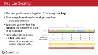
- 25. Key Cardinality • The best performance is gained from using row keys • Time range bound reads can skip store files • So can Bloom Filters • Selecting column families reduces the amount of data to be scanned • Pure value based access is a full table scan • Filters often are too, but reduce network traffic
- 26. Key/Table Design • Crucial to gain best performance • Why do I need to know? Well, you also need to know that RDBMS is only working well when columns are indexed and query plan is OK • Absence of secondary indexes forces use of row key or column name sorting • Transfer multiple indexes into one • Generate large table -> Good since fits architecture and spreads across cluster • DDI • Stands for Denormalization, Duplication and Intelligent Keys • Needed to overcome trade-offs of architecture • Denormalization -> Replacement for JOINs • Duplication -> Design for reads • Intelligent Keys -> Implement indexing and sorting, optimize reads
- 27. Pre-materialize Everything • Achieve one read per customer request if possible • Otherwise keep at lowest number • Reads between 10ms (cache miss) and 1ms (cache hit) • Use MapReduce or Spark to compute exacts in batch • Store and merge updates live • Use increment() methods Motto: “Design for Reads”
- 28. Tall-Narrow vs. Flat-Wide Tables • Rows do not split • Might end up with one row per region • Same storage footprint • Put more details into the row key • Sometimes dummy column only • Make use of partial key scans • Tall with Scans, Wide with Gets • Atomicity only on row level • Examples • Large graphs, stored as adjacency matrix (narrow) • Message inbox (wide)
- 29. Sequential Keys <timestamp><more key>: {CF: {CQ: {TS : Val}}} • Hotspotting on regions is bad! • Instead do one of the following: • Salting • Prefix <timestamp> with distributed value • Binning or bucketing rows across regions • Key field swap/promotion • Move <more key> before the timestamp (see OpenTSDB) • Randomization • Move <timestamp> out of key or prefix with MD5 hash • Might also be mitigated by overall spread of workloads
- 30. Key Design Choices • Based on access pattern, either use sequential or random keys • Often a combination of both is needed • Overcome architectural limitations • Neither is necessarily bad • Use bulk import for sequential keys and reads • Random keys are good for random access patterns
- 31. Checklist • Design for Use-Case • Read, Write, or Both? • Avoid Hotspotting • Hash leading key part, or use salting/bucketing • Use bulk loading where possible • Monitor your servers! • Presplit tables • Try prefix encoding when values are small • Otherwise use compression (or both) • For Reads: Restrict yourself • Specify what you need, i.e. columns, families, time range • Shift details to appropriate position • Composite Keys • Column Qualifiers
- 32. Performance Tuning 1000 knobs to turn… 20 are important?
- 33. Everything is Pluggable • Cell • Memstore • Flush Policy • Compaction Policy • Cache • WAL • RPC handling • …
- 34. Cluster Tuning • First, tune the global settings • Heap size and GC algorithm • Memory share for reads and writes • Enable Block Cache • Number of RPC handlers • Load Balancer • Default flush and compaction strategy • Thread pools (10+) • Next, tune the per-table and family settings • Region sizes • Block sizes • Compression and encoding • Compactions • …
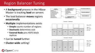
- 35. Region Balancer Tuning • A background process in the HBase Master is tracking load on servers • The load balancer moves regions occasionally • Multiple implementations exists • Simple counts number of regions • Stochastic determines cost • Favored Node pins HDFS block replicas • Can be tuned further • Cluster-wide setting!
- 36. RPC Tuning • Default is one queue for all types of requests • Can be split into separate queues for reads and writes • Read queue can be further split into reads and scans Stricter resource limits, but may avoid cross- starvation
- 37. Key Tuning • Design keys to match use-case • Sequential, salted, or random • Use sorting to convey meaning • Colocate related data • Spread load over all servers • Clever key design can make use of distribution: aging-out regions
- 38. Compaction Tuning • Default compaction settings are aggressive • Set for update use-case • For insert use-cases, Blooms are effective • Allows to tune down compactions • Saves resources by reducing write amplification • More store files are also enabling faster full table scans with time range bound scans • Server can ignore older files • Large regions may be eligible for advanced compaction strategies • Stripe or date-tiered compactions • Reduce rewrites to fraction of region size
- 39. Use-Cases What works well, what does not, and what is so-so
- 40. Placing the Use-Case • HBase chooses to work best for random access • You can optimize a table to prefer scans over gets • Fewer columns with larger payload • Larger HFile block sizes (maybe even duplicate data in two differently configured column families) • After that is the realm of hybrid systems • For fastest scans use brute force HDFS and native query engine with a columnar format
- 41. Big Data Workloads Low latency Batch Random Access Full ScanShort Scan HDFS + MR (Hive/Pig) HBase HBase + Snapshots -> HDFS + MR/Spark HDFS + SQL HBase + MR/Spark
- 42. Big Data Workloads Low latency Batch Random Access Full ScanShort Scan HDFS + MR/Spark (Hive/Pig) HBase HBase + Snapshots -> HDFS + MR/Spark HDFS + SQL HBase + MR/Spark Current Metrics Graph data Simple Entities Hybrid Entity Time series + Rollup serving Messages Analytic archive Hybrid Entity Time series + Rollup generation Index building Entity Time series
- 44. Optimizations Mostly Inserts Use-Cases • Tune down compactions • Compaction ratio, max store file size • Use Bloom Filters • On by default for row keys Mostly Update Use-Cases • Batch updates if possible Mostly Serial Keys • Use bulk loading or salting Mostly Random Keys • Hash key with MD5 prefix Mostly Random Reads • Decrease HFile block size • Use random keys Mostly Scans • Increase HFile (and HDFS) block size • Reduce columns and increase cell sizes
- 45. What matters… • For optimal performance, two things need to be considered: • Optimize the cluster and table settings • Choose the matching key schema • Ensure load is spread over tables and cluster nodes • HBase works best for random access and bound scans • HBase can be optimized for larger scans, but its sweet spot is short burst scans (can be parallelized too) and random point gets • Java heap space limits addressable space • Play with region sizes, compaction strategies, and key design to maximize result • Using HBase for a suitable use-case will make for a happy customer… • Conversely, forcing it into non-suitable use-cases may be cause for trouble
- 46. Questions?
Editor's Notes
- For Developers & End-Users – Apache Phoenix, Spark
- Importance of Row Key structure
- Time-series Data etc.
- Time-series Data etc.