Ism et chapter_3

−1/2 1
f (x0 ) = f (0) = (2 · 0 + 9) =
3
So,
L(x) = f (x0 ) + f (x0 ) (x − x0 )
1
= 3 + (x − 0)
3
Chapter 3 =3+ x
1
3
(b) Using √ the approximation L(x) to esti-
√
mate 8.8, we get 8.8 = f (−0.1) ≈
Applications of 1
L(−0.1) = 3 + (−0.1) = 3 − 0.033 =
3
2.967
Diﬀerentiation 4. (a) f (x) =
2
, x0 = 1
x
f (x0 ) = f (1) = 2
2
f (x) = − 2 and so f (1) = −2
x
3.1 Linear Approximations The linear approximation is
L(x) = 2 + (−2) (x − 1)
and Newtons Method
√ (b) Using the approximation L(x) to estimate
1. (a) f (x) = x, x0 = 1 2 2
√ , we get = f (0.99) ≈ L(0.99) =
f (x0 ) = f (1) = 1 = 1 0.99 0.99
1 2 + (−2)(0.99 − 1) = 2.02
f (x) = x−1/2
2
1 5. (a) f (x) = sin 3x, x0 = 0
f (x0 ) = f (1) = f (x0 ) = sin(3 · 0) = 0
2
So, f (x) = 3 cos 3x
L(x) = f (x0 ) + f (x0 ) (x − x0 ) f (x0 ) = f (0) = 3 cos(3 · 0) = 3
1 So,
= 1 + (x − 1) L(x) = f (x0 ) + f (x0 ) (x − x0 )
2
1 1 = 0 + 3 (x − 0)
= + x
2 2 = 3x
(b) √
Using the approximation L(x) to estimate
√ (b) Using the approximation L(x) to esti-
1.2, we get 1.2 = f (1.2) ≈ L(1.2) =
1 1 mate sin(0.3), we get sin(0.3) = f (0.1) ≈
+ (1.2) = 1.1 L(0.1) = 3(0.1) = 0.3
2 2
2. (a) f (x0 ) = f (0) = 1 and 6. (a) f (x) = sin x, x0 = π
1 −2/3
f (x0 ) = sin π = 0
f (x) = (x + 1)
3 f (x) = cos x
1
So, f (0) = f (x0 ) = f (π) = cos π = −1
3 The linear approximation is,
The Linear approximation is,
1 1 L(x) = f (x0 ) + f (x0 ) (x − x0 )
L(x) = 1 + (x − 0) = 1 + x
3 3 = 0 + (−1) (x − π) = π − x
(b) Using the approximation L(x) to estimate
√ √
3 3
(b) Using the approximation L(x) to esti-
1.2, we get 1.2 = f (0.2) ≈ L(0.2) = mate sin(3.0), we get sin(3.0) = f (3.0) ≈
1
1 + (0.2) = 1.066 L(3.0) = π − 3.0
3
√ √
4
3. (a) f (x) = 2x + 9, √0 = 0
x 7. (a) f (x) = √ 16 + x, x0 = 0
4
f (x0 ) = f (0) = 2 · 0+9 = 3 f (0) = 16 + 0 = 2
1 1
f (x) = (2x + 9)
−1/2
·2 f (x) = (16 + x)−3/4
2 4
1 1
= (2x + 9)
−1/2 f (0) = (16 + 0)−3/4 =
4 32

150

3.1. LINEAR APPROXIMATIONS AND NEWTONS METHOD 151

L(x) = f (0) + f (0)(x − 0) 36
L(72) = 120 + (72 − 80)
1 20
=2+ x = 120 + 1.8(−8)
32
1 = 105.6 cans
= 2 + (0.04) = 2.00125
32 168 − 120
1 (b) L(x) = f (100) + (x − 100)
(b) L(0.08) = 2 + (0.08) = 2.0025 100 − 80
32 48
1 L(94) = 168 − (94 − 100)
(c) L(0.16) = 2 + (0.16) = 2.005 20
32 = 168 − 2.4(−6)
8. (a) f (x) = sin x, x0 = 0 = 182.4 cans
f (0) = 0
f (x) = cos x 142 − 128
f (0) = cos 0 = 1 11. (a) L(x) = f (200) + (x − 200)
220 − 200
L(x) = f (0) + f (0) (x − 0) 14
L(208) = 128 + (208 − 200)
=0+1·x 20
L(0.1) = 0.1 = 128 + 0.7(8) = 133.6
(b) f (x) = sin x, x0 = π 142 − 136
√ 3
π 3 (b) L(x) = f (240) + (x − 240)
f = 220 − 240
3 2 6
π π 1 L(232) = 136 − (232 − 240)
f = cos = 20
3 3 2 = 136 − 0.3(−8) = 138.4
π π π
L(x) = f +f x−
√ 3 3 3
3 1 π 14 − 8
L(1) = + 1− ≈ 0.842 12. (a) L(x) = f (10) + (x − 10)
2 2 3 10 − 5
2π 6
(c) f (x) = sin x, x0 = L(8) = 14 + (−2) = 11.6
√ 3 5
2π 3 14 − 8
f = (b) L(x) = f (10) + (x − 10)
3 2 10 − 5
2π 2π 1 6
f = cos =− L(12) = 14 + (2) = 16.4
3 3 2 5
2π 2π 2π
L(x) = f +f x− 13. f (x) = x3 + 3x2 − 1 = 0, x0 = 1
3 3 3
√ f (x) = 3x2 + 6x
3 1 2π
= − x−
2√ 2 3
f (x0 )
9 3 1 9 2π (a) x1 = x0 −
L = − − ≈ 0.788 f (x0 )
4 2 2 4 3
13 + 3 · 12 − 1
18 − 14 =1−
9. (a) L(x) = f (20) + (x − 20) 3 · 12 + 6 · 1
20 − 30 3 2
4 =1− =
L(24) ≈ 18 − (24 − 20) 9 3
10 f (x1 )
= 18 − 0.4(4) x2 = x1 −
f (x1 )
= 16.4 games 2 3 2 2
2 3 +3 3 −1
14 − 12 = −
3 2 2 2
(b) L(x) = f (40) + (x − 40) 3 3 +6 3
30 − 40
2 79
f (36) ≈ 12 − (36 − 40) = ≈ 0.5486
10 144
= 12 − 0.2(−4) (b) 0.53209
= 12.8 games
120 − 84 14. f (x) = x3 + 4x2 − x − 1, x0 = −1
10. (a) L(x) = f (80) + (x − 80) f (x) = 3x2 + 8x − 1
80 − 60

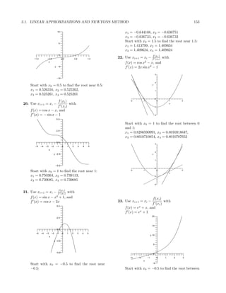
152 CHAPTER 3. APPLICATIONS OF DIFFERENTIATION

f (x0 ) 30
(a) x1 = x0 −
f (x0 )
3 1
= −1 − =− 20
−6 2
f (x1 ) y
x2 = x1 −
f (x1 ) 10

1 0.375
=− − = −0.4117647
2 −4.25
0
−5.0 −2.5 0.0 2.5 5.0
(b) The root is x ≈ −0.4064206546. x
−10

Start with x0 = −5 to find the root near −5:
15. f (x) = x4 − 3x2 + 1 = 0, x0 = 1 x1 = −4.718750, x2 = −4.686202,
f (x) = 4x3 − 6x x3 = −4.6857796, x4 = −4.6857795

f (x0 )
(a) x1 = x0 − 18. From the graph, we see two roots:
f (x0 )
14 − 3 · 12 + 1 1
=1− = 15

4 · 13 − 6 · 1 2
10
f (x1 )
x2 = x1 −
f (x1 ) 5

-1 0 1 2 3 4
1 4 1 2 0
1 2 −3 2 +1
= −
2 1 3 1 -5
4 2 −6 2
-10
5
=
8 -15

-20

(b) 0.61803

16. f (x) = x4 − 3x2 + 1, x0 = −1 f (xi )
Use xi+1 = xi − with
f (x) = 4x3 − 6x f (xi )
f (x) = x4 − 4x3 + x2 − 1, and
f (x) = 4x3 − 12x2 + 2x
f (x0 ) Start with x0 = 4 to find the root below 4:
(a) x1 = x0 − x1 = 3.791666667, x2 = 3.753630030, x3 =
f (x0 )
−1 1 3.7524339, x4 = 3.752432297
= −1 − =− Start with x = −1 to find the root just above
2 2
f (x1 ) −1:
x2 = x1 − x1 = −0.7222222222,
f (x1 )
x2 = −0.5810217936,
1 0.3125 x3 = −0.5416512863,
=− − = −0.625
2 2.5 x4 = −0.5387668233,
x5 = −0.5387519962
(b) The root is x ≈ −0.6180339887.

f (xi ) f (xi )
17. Use xi+1 = xi − with 19. Use xi+1 = xi − with
f (xi ) f (xi )
f (x) = x3 + 4x2 − 3x + 1, and f (x) = x5 + 3x3 + x − 1, and
f (x) = 3x2 + 8x − 3 f (x) = 5x4 + 9x2 + 1


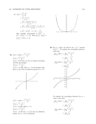
10 x1 = −0.644108, x2 = −0.636751
x3 = −0.636733, x4 = −0.636733
Start with x0 = 1.5 to find the root near 1.5:
5
x1 = 1.413799, x2 = 1.409634
x3 = 1.409624, x4 = 1.409624
0

−1.0 −0.5 0.0 0.5 1.0
22. Use xi+1 = xi − f (xii)) with
f
(x
x
f (x) = cos x2 − x, and
y −5 f (x) = 2x sin x2 − 1
3

−10

2
Start with x0 = 0.5 to find the root near 0.5: y

x1 = 0.526316, x2 = 0.525262, 1

x3 = 0.525261, x4 = 0.525261
0
f (xi ) -2 -1 0 1 2

20. Use xi+1 = xi − with x
f (xi ) -1

f (x) = cos x − x, and
f (x) = − sin x − 1 -2

5.0

Start with x0 = 1 to find the root between 0
and 1:
2.5
x1 = 0.8286590991, x2 = 0.8016918647,
x3 = 0.8010710854, x4 = 0.8010707652
0.0
3
−5 −4 −3 −2 −1 0 1 2 3 4 5
x
2
y −2.5 y

1

−5.0
0
Start with x0 = 1 to find the root near 1: -2 -1 0 1
x
2

x1 = 0.750364, x2 = 0.739113, -1

x3 = 0.739085, x4 = 0.739085
-2

21. Use xi+1 = xi − f (xii)) with
f
(x
f (x) = sin x − x2 + 1, and f (xi )
f (x) = cos x − 2x 23. Use xi+1 = xi − with
f (xi )
5.0
f (x) = ex + x, and
f (x) = ex + 1
20
2.5

15
0.0

−5 −4 −3 −2 −1 0 1 2 3 4 5
y 10
x

y −2.5
5

−5.0
0

−3 −2 −1 0 1 2 3
x
Start with x0 = −0.5 to find the root near −5

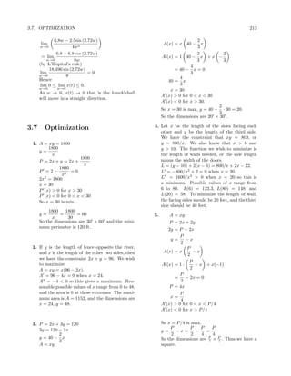
−0.5: Start with x0 = −0.5 to find the root between


0 and -1: zeros of f ), Newton’s method will succeed.
x1 = −0.566311, x2 = −0.567143 Which root is found depends on the starting
x3 = −0.567143, x4 = −0.567143 place.
f (xi ) 33. f (x) = x2 + 1, x0 = 0
24. Use xi+1 = xi − with
√ f (xi ) f (x) = 2x
f (x) = e−x − x, and f (x0 ) 1
1 x1 = x0 − =0−
f (x) = −e−x − √ f (x0 ) 0
2 x The method fails because f (x0 ) = 0. There
are no roots.
1
34. Newton’s method fails because the function
0.5
does not have a root!
4x2 − 8x + 1
0
0 0.5 1 1.5 2
35. f (x) = = 0, x0 = −1
4x2 − 3x − 7
Note: f (x0 ) = f (−1) is undefined, so New-
-0.5
ton’s Method fails because x0 is not in the do-
main of f . Notice that f (x) = 0 only when
-1
4x2 − 8x + 1 = 0. So using Newton’s Method
on g(x) = 4x2 − 8x + 1 with x0 = −1 leads to
x ≈ .1339. The other root is x ≈ 1.8660.
Start with x0 = 0.5 to find the root close to
36. The slope tends to infinity at the zero. For ev-
0.5:
ery starting point, the sequence does not con-
x1 = 0.4234369253, x2 = 0.4262982542,
verge.
x3 = 0.4263027510
√ 37. (a) With x0 = 1.2,
25. f (x) = x2 − 11; x0 = 3; 11 ≈ 3.316625
√ x1 = 0.800000000,
26. Newton’s method for x near x = 23 is xn+1 = x2 = 0.950000000,
1
2 (xn + 23/xn ). Start with x0 = 5 to get:
x3 = 0.995652174,
x1 = 4.8, x2 = 4.7958333, and x3 = 4.7958315. x4 = 0.999962680,
√ x5 = 0.999999997,
27. f (x) = x3 − 11; x0 = 2; 3 11 ≈ 2.22398 x6 = 1.000000000,
√ x7 = 1.000000000
28. Newton’s method for 3 x near x = 23 is
xn+1 = 1 (2xn + 23/x2 ). Start with x0 = 3
3 n (b) With x0 = 2.2,
to get: x0 = 2.200000, x1 = 2.107692,
x1 = 2.851851851, x2 = 2.843889316, and x2 = 2.056342, x3 = 2.028903,
x3 = 2.884386698 x4 = 2.014652, x5 = 2.007378,
√ x6 = 2.003703, x7 = 2.001855,
29. f (x) = x4.4 − 24; x0 = 2; 4.4 24 ≈ 2.059133
x8 = 2.000928, x9 = 2.000464,
√
30. Newton’s method for 4.6 x near x = 24 is x10 = 2.000232, x11 = 2.000116,
1
xn+1 = 4.6 (3.6xn +24/x3.6 ). Start with x0 = 2
n x12 = 2.000058, x13 = 2.000029,
to get: x14 = 2.000015, x15 = 2.000007,
x1 = 1.995417100, x2 = 1.995473305, and x16 = 2.000004, x17 = 2.000002,
x3 = 1.995473304 x18 = 2.000001, x19 = 2.000000,
x20 = 2.000000
31. f (x) = 4x3 − 7x2 + 1 = 0, x0 = 0 The convergence is much faster with x0 =
f (x) = 12x2 − 14x 1.2.
f (x0 ) 1
x1 = x0 − =0−
f (x0 ) 0 38. Starting with x0 = 0.2 we get a sequence that
The method fails because f (x0 ) = 0. Roots converges to 0 very slowly. (The 20th itera-
are 0.3454, 0.4362, 1.659. tion is still not accurate past 7 decimal places).
Starting with x0 = 3 we get a sequence that
32. Newton’s method fails because f = 0. As long
7 quickly converges to π. (The third iteration is
as the sequence avoids xn = 0 and xn = (the already accurate to 10 decimal places!)
6


√
39. (a) With x0 = −1.1 43. f (x) = √ 4 + x
x1 = −1.0507937, f (0) = 4 + 0 = 2
x2 = −1.0256065, 1
f (x) = (4 + x)−1/2
x3 = −1.0128572, 2
1 1
x4 = −1.0064423, f (0) = (4 + 0)−1/2 =
x5 = −1.0032246, 2 4
1
x6 = −1.0016132, L(x) = f (0) + f (0)(x − 0) = 2 + x
4
x7 = −1.0008068, 1
x8 = −1.0004035, L(0.01) = 2 + (0.01) = 2.0025
√ 4
x9 = −1.0002017, f (0.01) = 4 + 0.01 ≈ 2.002498
x10 = −1.0001009, 1
L(0.1) = 2 + (0.1) = 2.025
x11 = −1.0000504, √ 4
x12 = −1.0000252, f (0.1) = 4 + 0.1 ≈ 2.0248
x13 = −1.0000126, 1
L(1) = 2 + (1) = 2.25
x14 = −1.0000063, √ 4
x15 = −1.0000032, f (1) = 4 + 1 ≈ 2.2361
x16 = −1.0000016,
x17 = −1.0000008,
x18 = −1.0000004,
x19 = −1.0000002,
x20 = −1.0000001, 44. The linear approximation for ex at x = 0 is
x21 = −1.0000000, L(x) = 1 + x. The error when x = 0.01 is
x22 = −1.0000000 0.0000502, when x = 0.1 is 0.00517, and when
(b) With x0 = 2.1 x = 1 is 0.718.
x0 = 2.100000000,
x1 = 2.006060606,
x2 = 2.000024340,
x3 = 2.000000000,
x4 = 2.000000000 45. (a) f (0) = g(0) = h(0) = 1, so all pass
The rate of convergence in (a) is slower through the point (0, 1).
than the rate of convergence in (b). f (0) = 2(0 + 1) = 2,
g (0) = 2 cos(2 · 0) = 2, and
40. From exercise 37, f (x) = (x − 1)(x − 2)2 . New-
h (0) = 2e2·0 = 2,
ton’s method converges slowly near the double
so all have slope 2 at x = 0.
root. From exercise 39, f (x) = (x − 2)(x + 1)2 .
The linear approximation at x = 0 for all
Newton’s method again converges slowly near
three functions is L(x) = 1 + 2x.
the double root. In exercise 38, Newton’s
method converges slowly near 0, which is a zero
of both x and sin x but converges quickly near
π, which is a zero only of sin x. (b) Graph of f (x) = (x + 1)2 :
5
41. f (x) = tan x, f (0) = tan 0 = 0
f (x) = sec2 x, f (0) = sec2 0 = 1 4

L(x) = f (0) + f (0)(x − 0) L(0.01) = 0.01
3
= 0 + 1(x − 0) = x y

f (0.01) = tan 0.01 ≈ 0.0100003 2

L(0.1) = 0.1 1
f (0.1) = tan(0.1) ≈ 0.1003
L(1) = 1 0

f (1) = tan 1 ≈ 1.557 −3 −2 −1 0 1 2 3
−1
√ x
42. The linear approximation for 1 + x at x = 0
1
is L(x) = 1 + 2 x. The error when x = 0.01 is
0.0000124, when x = 0.1 is 0.00119, and when
x = 1 is 0.0858. Graph of f (x) = 1 + sin(2x):


5
2

4

1
3
y
2 0
-2 -1 0 1 2
x
1
-1

0
−3 −2 −1 0 1 2 3
-2
x −1

Graph of h(x) = sinh x:

Graph of f (x) = e2x :
3
5
2

4
1

3 0
-2 -1 0 1 2
y
-1 x
2

-2

1
-3

0

−3 −2 −1 0 1 2 3
x −1
sin x is the closest ﬁt, but sinh x is close.

√
4
47. (a) 16.04 = 2.0012488
L(0.04) = 2.00125
|2.0012488 − 2.00125| = .00000117
46. (a) f (0) = g(0) = h(0) = 0, so all pass √
4
through the point (0, 0). (b) 16.08 = 2.0024953
f (0) = cos 0 = 1, L(.08) = 2.0025
1 |2.0024953 − 2.0025| = .00000467
g (0) = = 1, and
1 + 02 √
h (0) = cosh 0 = 1, (c) 4
16.16 = 2.0049814
so all have slope 1 at x = 0. L(.16) = 2.005
The linear approximation at x = 0 for all |2.0049814 − 2.005| = .0000186
three functions is L(x) = x.

(b) Graph of f (x) = sin x: 48. If you graph | tan x − x|, you see that the dif-
ference is less than .01 on the interval −.306 <
2 x < .306 (In fact, a slightly larger interval
would work as well).
1

49. The ﬁrst tangent line intersects the x-axis at a
0
-2 -1 0 1 2 point a little to the right of 1. So x1 is about
x
1.25 (very roughly). The second tangent line
-1
intersects the x-axis at a point between 1 and
x1 , so x2 is about 1.1 (very roughly). Newton’s
-2 Method will converge to the zero at x = 1.
Starting with x0 = −2, Newton’s method con-
Graph of g(x) = tan−1 x: verges to x = −1.


f (x) = 2x − 1
3
3
At x0 =
2
2
2
y 3 3 1
f (x0 ) = − −1=−
1 2 2 4
and
3
-2 -1
0
0 1 2
f (x0 ) = 2 −1=2
x
2
-1 By Newton’s formula,
f (x0 ) 3 −1 13
x1 = x0 − = − 4 =
-2 f (x0 ) 2 2 8

Starting with x0 = 0.4, Newton’s method con- (b) f (x) = x2 − x − 1
verges to x = 1. f (x) = 2x − 1
5
At x0 = 3
3 2
5 5 1
f (x0 ) = − −1=
2 3 3 9
y
and
5 7
1 f (x0 ) = 2 −1=
3 3
0
By Newton’s formula,
-2 -1 0 1 2
f (x0 )
x x1 = x0 −
-1 f (x0 )
1
5 9 5 1 34
-2 = − 7 = − =
3 3
3 21 21

50. It wouldn’t work because f (0) = 0. x0 = 0.2 (c) f (x) = x2 − x − 1
works better as an initial guess. After jumping f (x) = 2x − 1
8
to x1 = 2.55, the sequence rapidly decreases At x0 = 5
2
toward x = 1. Starting with x0 = 10, it takes 8 8 1
f (x0 ) = − −1=−
several steps to get to 2.5, on the way to x = 1. 5 5 25
and
f (xn ) 8 11
51. xn+1 = xn − f (x0 ) = 2 −1=
f (xn ) 5 5
x2 − c
n By Newton’s formula,
= xn − f (x0 )
2xn x1 = x0 −
x2 c f (x0 )
= xn − n + 8 − 25 1
8 1 89
2xn 2xn = − 11 = + =
xn c 5 5 55 55
= + 5
2 2xn
1 c (d) From part (a),
= xn + F4 F7
2 xn sincex0 = , hence x1 = .
√ √ √ F3 F6
If x0 < a, then a/x0 > a, so x0 < a < From part (b),
a/x0 . F5 F9
√ since x0 = hence x1 = .
52. The root of xn − c is n c, so Newton’s method F4 F8
From part (c),
approximates this number. F6 F11
Newton’s method gives since x0 = hence x1 = .
f (xi ) xn − c F5 F10
xi+1 = xi − = xi − i n−1 Fn+1
f (xi ) nxi Thus in general if x0 = , then x1 =
Fn
1 F2n+1
= (nxi − xi + cx1−n ),
i implies m = 2n + 1 and k = 2n
n F2n
as desired.
3 Fn+1
53. (a) f (x) = x2 − x − 1 (e) Given x0 = , then lim will be
2 n→∞ Fn


the zero of the function f (x) = x2 − 2P x
L(x) = 120 − .01(120) = P −
x − 1 which is 1.618034. Therefore, R
Fn+1 2 · 120x
lim = 1.618034 = 120 −
n→∞ Fn R
2x
.01 =
54. The general form of functionf (x) is, R
1 n+2 1 1 x = .005R = .005(20,900,000)
fn (x) = 2 x − 3 for n < x < n−1 .
5 2 2 = 104,500 ft
Hence
2n+2 1 1 58. If m = m0 (1 − v 2 /c2 )1/2 , then
f (x) = fn (x) = for n < x < n−1 .
5 2 2 m = (m0 /2)(1 − v 2 /c2 )−1/2 (−2v/c2 ), and
By Newton’s method,
m = 0 when v = 0. The linear approxima-
3 f 34 3 f1 34
x1 = − = − tion is the constant function m = m0 for small
4 f 3 4
4 f1 4 3
values v.
3 (3/5 ) 3 x0
= − = = 59. The only positive solution is 0.6407.
4 (8/5 ) 8 2
x1 x0 x0
Similarly, x2 = = 2 and x3 = 3 60. The smallest positive solution of the first equa-
2 2 2 tion is 0.132782, and for the second equa-
x0
Continuing this, we get, xn−1 = n−1 It may tion the smallest positive solution is 1, so the
2
also be observed that, for each fn (x) species modeled by the second equation is cer-
(1/2n ) + 1/2n+1 3 tain to go extinct. This is consistent with the
x0 = = n+1 ,
2 2 models, since the expected number of offspring
x0 3 3 for the population modeled by the first equa-
xn = n = 2n+1 ⇒ xn+1 = 2n+2 which
2 2 2 tion is 2.2, while for the second equation it is
is the zero of F . Therefore Newton’s method
only 1.3
converges to zero of F .
61. The linear approximation for the inverse tan-
55. For small x we approximate ex by x + 1 gent function at x = 0 is
(see exercise 44) f (x) ≈ f (0) + f (0)(x − 0)
Le2πd/L − e−2πd/L tan−1 (x) ≈ tan−1 (0) + 1+02 (x − 0)
1

e2πd/L + e−2πd/L tan−1 (x) ≈ x
L 1 + 2πd − 1 − 2πd
L L
Using this approximation,
≈ 3[1 − d/D] − w/2
1 + 2πd + 1 − 2πd
L L φ = tan−1
4πd
D−d
L L
≈ = 2πd 3[1 − d/D] − w/2
2 φ≈
4.9 D−d
f (d) ≈ · 2πd = 9.8d If d = 0, then φ ≈ 3−w/2 . Thus, if w or D
π D
increase, then φ decreases.
8πhcx−5
56. If f (x) = , then using the linear 62. d (θ) = D(w/6 sin θ)
ehc/(kT x) − 1 d(0) = D(1 − w/6) so
approximation we see that
8πhcx−5 d(θ) ≈ d(0) + d (0)(θ − 0)
f (x) ≈ hc
= 8πkT x−4 = D(1 − w/6) + 0(θ) = D(1 − w/6),
(1 + kT x ) − 1
as desired. as desired.

P R2
57. W (x) =
(R + x)2
, x0 = 0 3.2 Indeterminate Forms and
W (x) =
−2P R2 L’Hˆpital’s Rule
o
(R + x)3
L(x) = W (x0 ) + W (x0 )(x − x0 ) x+2
1. lim
x→−2 x2 − 4
P R2 −2P R2 x+2
= + (x − 0) = lim
(R + 0)2 (R + 0)3 x→−2 (x + 2)(x − 2)
2P x 1 1
=P− = lim =−
R x→−2 x − 2 4

ˆ
3.2. INDETERMINATE FORMS AND L’HOPITAL’S RULE 159

x2 − 4 sin x − x 0
2. lim 11. lim 3
is type ;
x→2 x2− 3x + 2 x→0 x 0
(x − 2)(x + 2) we apply L’Hˆpital’s Rule thrice to get
o
= lim cos x − 1 − sin x
x→2 (x − 2)(x − 1) = lim = lim
x+2 x→0 3x2 x→0 6x
= lim =4 − cos x 1
x→2 x − 1 = lim =− .
x→0 6 6
3x2 + 2
3. lim tan x − x 0
x→∞ x2 − 4 12. lim is type ;
2
3 + x2
x→0 x3 0
= lim we apply L’Hˆpital’s Rule to get
o
x→∞ 1 − 4 sec2 x − 1
x2
3 lim .
= =3 x→0 3x2
1
Apply L’Hˆpital’s Rule twice more to get
o
x+1 ∞ 2 sec2 x tan x
4. lim is type ; lim
x→−∞ x2 + 4x + 3 ∞ x→0 6x
4 sec2 x tan2 x + 2 sec4 x 1
we apply L’Hˆpital’s Rule to get
o = lim = .
1 x→0 6 3
lim = 0. √ √ √
x→−∞ 2x + 4
t−1 t−1 t+1
13. lim = lim · √
e2t − 1 0 t→1 t − 1 t→1 t − 1 t+1
5. lim is type ;
t→0 t 0 (t − 1)
o = lim √
t→1 (t − 1) t + 1
d
e2t − 1
lim dt d 1 1
= lim √ =
dt t
t→0
t→1 t+1 2
2e2t 2
lim = =2 ln t 0
t→0 1 1 14. lim is type ;
sin t 0
t→1 t −1 0
6. lim is type ;
t→0 e3t−1 0 we apply L’Hˆpital’s Rule to get
o
o d 1
dt (ln t)
d
(sin t) cos t 1 lim d = lim t = 1
t→1 1
dt (t − 1)
t→1
lim ddt 3t = lim 3t =
t→0 3e 3
dt (e − 1)
t→0
x3 ∞
tan−1 t 0 15. lim x is type ;
7. lim is type ; x→∞ e ∞
t→0 sin t 0 we apply L’Hˆpital’s Rule thrice to get
o
o
d
tan−1 t 1/(1 + t2 ) 3x2 6x
lim dt d = lim =1 lim = lim x
t→0
dt (sin t)
t→0 cos t x→∞ ex x→∞ e
6
sin t 0 = lim x = 0.
8. lim is type ; x→∞ e
t→0 sin−1 t 0
ex ∞
o 16. lim is type ;
d x→∞ x4 ∞
dt (sin t) cos t
lim = lim √ =1 we apply L’Hˆpital’s Rule four times to get
o
t→0 d sin−1 t t→0 1/( 1 − t2 )
dt ex ex
lim 3
= lim
sin 2x 0 x→∞ 4x x→∞ 12x2
9. lim is type ; ex ex
x→π sin x 0 = lim = lim = ∞.
x→∞ 24x x→∞ 24
o
x cos x − sin x ∞
2 cos 2x 2(1) 17. limx→0 2 is type ;
lim = = −2. x sin x ∞
x→π cos x −1 we apply L’Hˆpital’s Rule twice to get
o
cos x − x sin x − cos x
cos−1 x limx→0
10. lim is undeﬁned (numerator goes to sin2 x + 2x sin x cos x
x→−1 x2 − 1 −x sin x
π, denominator goes to 0). = lim
x→0 sin x (sin x + 2x cos x)


−x x − π cos x
= lim = lim 2
= 0
x→0 sin x + 2x cos x
−1
π
x→ 2 cos x − x − π sin x
2
= lim
x→0 cos x + 2 cos x − 2x sin x ln x ∞
1 21. lim 2 is type
=− . x→∞ x ∞
3 we apply L’Hˆpital’s Rule to get
o
1/x 1
18. Rewrite as one fraction, we have lim = lim = 0.
x→∞ 2x x→∞ 2x2
1 x cos x − sin x
lim cot x − = lim ln x ∞
x→0 x x→0 x sin x 22. lim √ is type ;
0 x→∞ x ∞
which is of type we apply L’Hˆpital’s Rule to get
o
0 1
o 2
cos x − x sin x − cos x lim x = lim √ = 0.
1
= lim
x→∞ √
2 x
x→∞ x
x→0 sin x + x cos x
t ∞
d
(−x sin x) 23. lim t is type
= lim dx t→∞ e ∞
x→0 d
(sin x + x cos x) we apply L’Hˆpital’s Rule to get
o
dx d
(t) 1
− sin x − x cos x lim dt = lim t = 0.
= lim =0 t→∞ d (et ) t→∞ e
x→0 cos x + cos x − x sin x dt

sin 1
t 0
19. Rewrite as one fraction, we have 24. lim 1 is type
t→∞
t
0
x+1 2 we apply L’Hˆpital’s Rule to get
o
lim −
x→0 x sin 2x - 1 cos 1
2 1
(x + 1) sin 2x − 2x 0 = lim t 1 t = lim cos = 1.
= lim is type ; t→∞ − t2 t→∞ t
x→0 x sin 2x 0
we apply L’Hˆpital’s Rule four times to get
o ln (ln t)
d 25. lim
(x + 1) sin 2x − 2x t→1 ln t
lim dx d As t approaches ln from below, ln t is a small
dx (x sin 2x)
x→0
negative number. Hence ln (ln t) is undeﬁned,
sin 2x + 2(x + 1) cos 2x − 2 so the limit is undeﬁned.
= lim
x→0 sin 2x + 2x cos 2x
d
sin (sin t) 0
(sin 2x + 2(x + 1) cos 2x − 2) 26. lim is type
= lim dx d t→0 sin t 0
dx (sin 2x + 2x cos 2x)
x→0 we apply L’Hˆpital’s Rule to get
o
2 cos 2x + 2 cos 2x − 4(x + 1) sin 2x cos (sin t) cos t
= lim lim = 1.
x→0 2 cos 2x + 2 cos 2x − 4x sin 2x t→0 cos t
4
= =1 sin (sinh x) 0
4 27. lim is type
x→0 sinh (sin x) 0
o
1 cos (sinh x) cosh x
20. lim tan x + lim =1
π
x→ 2 x− π 2
x→0 cosh (sin x) cos x
In this case the limit has the form (∞ - ∞). sin x − sinh x
sin x 28. lim
Rewrite tan x as and then as one frac- x→0 cos x − cosh x
cos x
tion, we get 2 sin x − ex + e−x
= lim
1 x→0 2 cos x − ex − e−x
lim tan x +
x→ 2π
x− π 2
2ex sin x − e2x + 1 0
= lim is type
sin x 1 x→0 2ex cos x − e2x − 1 0
= lim + we apply L’Hˆpital’s Rule twice to get
o
x→ π
2 cos x x − π 2
2ex cos x + 2ex sin x − 2e2x
x − π sin x + cos x
2 0 lim
= lim is type x→0 −2ex sin x + 2ex cos x − 2e2x
x→ π
2 x − π cos x
2
0
cos x + sin x − 1 0
o = lim is type
x→0 cos x − sin x − 1 0
sin x + x − π cos x − sin x
2 − sin x + cos x
= lim = lim = −1
x→ π
2 cos x − x − π sin x
2 x→0 − sin x − cos x

ˆ

ln x ∞ x+1
 
29. lim is type
x→0 + cot x ∞  ln x−2 
o = lim  
x→∞  √ 1 
1/x x2 −4
lim
x→0+ − csc2 x 0
sin x This last limit has indeterminate form , so
= lim+ − sin x · = (0)(1) = 0. 0
x→0 x we can apply L’Hˆpital’s Rule and simplify to
o
ﬁnd that the above is equal to
√
x −3(x2 − 4)3/2
30. lim+ = 0 (numerator goes to 0 and de- lim and this is equal to 3. So
x→0 ln x x→∞ −x3 + x2 + 2x
nominator goes to −∞). lim ln y = 3.
x→∞
Thus lim y = lim eln y = e3 ≈ 20.086.
x→∞ x→∞
31. lim x2 + 1 − x √
x→∞
√ 1 x
x2 + 1 + x 35. lim+ √ −√
= lim x 2+1−x √ x→0 x√ x+1 √
x→∞ x2 + 1 + x x + 1 − ( x)2
2
x +1−x 2 = lim+ √ √
= lim √ x→0
√ x x+1
x→∞ x2 + 1 + x x+1−x
1 = lim √ √
= lim √ =0 x→0+ x x+1
x→∞ x 2+1+x = ∞.
√
5−x−2 0
ln x
−1 36. lim √ is type
32. lim ln x − x = lim x
= −∞ since the x→1 10 − x − 3 0
1
x→∞ x→∞
x
o
numerator goes to −1 and the denominator 1 −1/2
2 (5 − x) (−1)
goes to 0+ . (Recall Example 2.8 which shows lim 1
x→1 (10 − x)−1/2 (−1)
2 √
ln x
lim = 0.) 10 − x 3
x→∞ x = lim √ = .
x→1 5−x 2
x x
1 37. Let y = (1/x) . Then ln y = x ln(1/x). Then
33. Let y = 1+
x lim+ ln y = lim+ x ln(1/x) = 0, by Exercise
x→0 x→0
1
⇒ ln y = x ln 1 + . Then 27. Thus lim+ y = lim+ eln y = 1.
x x→0 x→0
1
lim ln y = lim x ln 1 + 38. Let y = lim+ (cos x)1/x . Then
x→∞ x→∞ x x→0
ln 1 + x 1 1
= lim ln y = lim+ ln cos x
x→0 x
x→∞ 1/x
1 1 ln(cos x) 0
1+ x1 − x2 = lim is type
= lim x→0 + x 0
x→∞ −1/x2 so apply L’Hˆpital’s Rule to get
o
1 − tan x
= lim = 1. lim+ = 0.
x→∞ 1 + 1 x→0 1
x
Hence lim y = lim eln y = e. Therefore the limit is y = e0 = 1.
x→∞ x→∞
t t
t−3 (t − 3)
39. lim = lim
34. Notice that the limit in question has the inde- t→∞ t+2 t→∞ (t + 2)t
terminate form 1∞ . Also, note that as x gets 3 t lim 1 − 3
t
x+1 x+1 1− t t→∞ t
large, = . = lim =
t→∞ 2 t 2 t
x−2 x −√2 1+ t lim 1 + t
t→∞
x2 −4 −3 t
x+1 lim 1 +
Deﬁne y = . Then t→∞ t e−3
x−2 = = = e−5
2 t e2
√ x+1 lim 1 + t
t→∞
ln y = x2 − 4 ln and
x−2 t t
3
x+1 t−3 1− t
lim ln y = lim x2 − 4 ln 40. lim = lim 1
x→∞ x→∞ x−2 t→∞ 2t + 1 t→∞ 2+ t


3 t
1− t e−3 we apply L’Hˆpital’s Rule to get
o
= lim t = lim =0
t→∞ 1/2 t→∞ 2t e1/2
2t 1 + n cos nx n
t lim = .
x→0 m cos mx m
41. L’Hˆpital’s rule does not apply. As x → 0, the
o sin x2 2x cos x2
numerator gets close to 1 and the denominator 50. (a) lim 2
= lim
x→0 x x→0 2x
is small and positive. Hence the limit is ∞.
= lim cos x2 = 1,
ex − 1 0 ex x→0
42. lim is type , but lim is not, so sin x
x→0 x 2 0 x→0 2x which is the same as lim .
L’Hˆpital’s Rule does not apply to this limit.
o x→0 x

1 − cos x2
43. L’Hˆpital’s rule does not apply. As x → 0, the
o (b) lim
x→0 x4
numerator is small and positive while the de- 2x sin x2 sin x2
nominator goes to −∞. Hence the limit is 0. = lim 3
= lim
x→0 4x x→0 2x2
2x 1 sin x 2
1
Also lim , which equals lim x2 , is not of = lim = (by part (a)),
x→0 2/x x→0
2 x→0 x2 2
0
the form so L’Hˆpital’s rule doesn’t apply
o
0 while
here either.
sin x 0 cos x 1 − cos x sin x 1 1
44. lim is type , but lim is not, so lim 2
= lim = (1) =
x→0 x2 0 x→0 2x x→0 x x→0 2x 2 2
L’Hˆpital’s rule does not apply. This limit is
o so both of these limits are the same.
undefined because the numerator goes to 1 and (c) Based on the patterns found in exercise
the denominator goes to 0. 45, we should guess
csc x sin x3 1 − cos x3 1
45. lim+ √ lim = 1 and lim = .
x→0 x x→0 x3 x→0 x6 2
∞
In this case limit has the form , L’Hˆspital’s
o
0 (x + 1)(2 + sin x)
Rule should not be used. 51. (a)
x(2 + cos x)
x−3/2 ∞ x
46. lim+ is type . In this case (b) x
x→0 ln x −∞ e
L’Hˆspital’s Rule should be used.
o 3x + 1
(c)
x2 − 3x + 1 x−7
47. lim = ∞. In this case limit has 3 − 8x
x→∞ tan−1 x (d)
the form ∞. So L’Hˆspital’s Rule should not
o 1 + 2x
be used.
52. (a) lim x − ln x = ∞ (see exercise 32).
ln x2 ∞ x→∞
48. lim is type . So L’Hˆspital’s Rule
o √
x→∞ ex/3 ∞ (b) lim x2 + 1 − x = 0 (see exercise 31).
should be used. x→∞
√
sin 3x (c) lim x2 + 4x − x
49. (a) Starting with lim , we cannot x→∞ √
sin 2x
x→0 = lim ( x2 + 4x − x)
3x x→∞
“cancel sin”to get lim . We can cancel 4x
x→0 2x = lim √
the x’s in the last limit to get the final an- x→∞ x2 + 4x + x
swser of 3/2. The first step is likely to give 1
4x x
a correct answer because the linear ap- = lim √
x→∞ 1
proximation of sin 3x is 3x, and the linear ( x2 + 4x + x)
x
approximation of sin 2x is 2x. The linear 4
= lim = 2,
approximations are better the closer x is x→∞ 4
1+ x +1
to zero, so the limits are likely to be the
where to get from the second to
same.
the third line, we have multiplied by
√
sin nx
(b) lim is type 0 ;
0
( x2 + 4x + x)
x→0 sin mx √ .
( x2 + 4x + x)

ˆ

53. lim ex = lim xn = ∞ In general,when the degree of exponential term
x→∞ x→∞
ex in the numerator and denominator are diﬀer-
lim n = ∞. Since n applications of ln ekx + p(x)
x→∞ x ent, then the lim for polyno-
L’Hˆpital’s rule yields
o x→∞ ln (ecx + q(x))
ex mials p and q and positive numbers. k and c
lim = ∞.
x→∞ n! will be the fraction of degrees that is k .
c
Hence e dominates xn .
x

54. lim ln x = lim xp = ∞. 59. If x → 0, then x2 → 0, so if lim
f (x)
= L,
x→∞ x→∞
ln x ∞ x→0 g(x)
lim is of type f (x2 )
x→∞ xp ∞ then lim = L (but not conversely). If
we use L’Hˆpital’s Rule to get
o x→0 g(x2 )
1
x 1 f (x)
lim p−1
= lim = 0 (since p > 0). a = 0 or 1, then lim involves the be-
x→∞ px x→∞ pxp x→a g(x)
p
Therefore, x dominates ln x. f (x2 )
havior of the quotient near a, while lim
t t
x→a g(x2 )
55. lim e 2 − t3 Since e 2 dominates t3 . So involves the behavior of the quotient near the
t→∞
t diﬀerent point a2 .
lim e − t3 = ∞
2
t→∞
60. Functions f (x) = |x| and g(x) = x work.
√ f (x)
x − ln x ∞ lim does not exist as it approaches −1
56. lim √ is type . x→0 g(x)
x→∞ x ∞
from the left and it approaches 1 from the
o
√ − 1
1 √ f (x2 )
2 x x x−2 x right, but lim = 1.
lim = lim x→0 g(x2 )
x→∞ 1
√ x→∞ x
2 x
2 2.5(4ωt − sin 4ωt)
= lim 1 − √ = 1. 61. lim
x→∞ x ω→0 4ω 2
2.5(4t − 4t cos 4ωt)
= lim
ln x3 + 2x + 1
ω→0 8ω
57. lim 2.5(16t2 sin 4ωt)
x→∞ ln (x2 + x + 2) = lim =0
ω→0 8
we apply L’Hˆpital’s Rule
o
d
dx ln x3 + 2x + 1 π
lim 2.5 − 2.5 sin(4ωt + )
d 2 2 is type 0 ;
dx (ln (x + x + 2))
x→∞
62. lim 0
3x2 +2
ω→0 4ω 2
x3 +2x+1 we apply L’Hˆpital’s Rule to get
o
= lim 2x+1 −10t cos(4ωt + π )
x→∞ 2
x2 +x+2 lim
3x + 3x + 8x2 + 2x + 4
4 3
3 ω→0 8ω
= lim = 40t2 sin(4ωt + π )
x→∞ 2x 4 + x3 + 4x2 + 4x + 1 2 = lim 2
= 5t2 .
In general, for numerator and denominator the
ω→0 8
highest degee of polynomials p and q, such that
p(x) > 0 and q(x) > 0 for x > 0, 2

should be the lim ln(p(x)) .
ln(q(x))
x→∞
1.5

3x
ln e + x ∞
58. lim 2x + 4)
is ; 1
x→∞ ln (e ∞
we apply L’Hˆpital’s Rule
o 0.5
d 3x
dx ln e +x
lim d
x→∞
dx (ln (e2x + 4)) 0
0 0.1 0.2 0.3 0.4 0.5 0.6
3e3x +1 t
e3x +x
= lim 2e2x
x→∞
e2x +4
5x
3e + 12e3x + e2x + 4 3 63. The area of triangular region 1 is
= lim = (1/2)(base)(height)
x→∞ 2e5x + 2xe2x 2


= (1/2)(1 − cos θ)(sin θ). (b) lim V
m→0 √ √
Let P be the center of the circle. The area of g g

region 2 equals the area of sector AP C minus e 40m t
− e− 40m t
= lim 40mg √ g √ g
the area of triangle AP B. The area of the m→0
e 40m t √ e− 40m t
+
g
sector is θ/2, while the area of triangle AP B 1 − e−2 40m t
is = lim 40mg √ g
(1/2)(base)(height)
m→0
1 + e−2 40m√ t
g
= (1/2)(cos θ)(sin θ). 1 − e−2 40m t
= lim 40mg lim √ g
Hence the area of region 1 divided by the area m→0 m→0
1 + e−2 40m t
of region 2 is =0
(1/2)(1 − cos θ)(sin θ) as m → 0; 2 40m t → ∞ andg

θ/2 − (1/2)(cos θ)(sin θ) √ g
e−2 40m t → 0. This means, when the
(1 − cos θ)(sin θ)
= mass is negligible, its velocity is 0.
θ − cos θ sin θ
sin θ − cos θ sin θ
=
θ − cos θ sin θ
sin θ − (1/2) sin 2θ
= (c) lim V
θ − (1/2) sin 2θ m→∞ √ g √ g
sin θ − (1/2) sin 2θ e 40m t − e− 40m t
Then limθ→0 = lim 40mg √ g √ g
θ − (1/2) sin 2θ
cos θ − cos 2θ
m→∞
e √ t + e− 40m t
40m

= lim g
e2 40m t − 1
θ→0 1 − cos 2θ
− sin θ + 2 sin 2θ = lim 40mg √ g
m→∞
= lim e2 40m t + 1
θ→0 2 sin 2θ g
as m → ∞; 2 40m t → 0 and
− cos θ + 4 cos 2θ √ g
= lim e2 40m t → 1
θ→0 4 cos 2θ √ g
−1 + 4(1) 3
1 e2 40m t − 1
= = √ g
4(1) 4 = lim lim √
m→∞
e2 40m t + 1 √ m→∞ 1/ 40mg
g
160x−0.4 + 90
2
e √
t
40m −1 √
= (1/2 ) √ lim 2 gt
64. lim+ g
(2 40m t)→0
g
2 40m t
x→0 8x−0.4 + 10 √
160 + 90x0.4 160 = gt
= lim = = 20. If there This means, when the increases indeﬁ-
x→0+ 8 + 10x0.4 8 √
is no light, the pupils will expand to this nitely, its velocity reaches gt.
size. This is the largest the pupils can get.
160x−0.4 + 90 90
lim = = 9. As the amount
x→∞ 8x−0.4 + 10 10
of light grows, the pupils shrink, and the size
approaches 6mm in the limit. This is the small-
est possible size of the pupils.
3/2
√ 66. lim S = lim 8π 2 d2
−1
3 c +1
g
65. (a) V = 40mg tanh 40m t , therefore c→∞ c→∞ 16c2
lim V c2 (d2 +16c2 )
3/2
−64c3
t→∞ √ √ 8π
g g = lim
3 c→∞ 64c3
e 40m t
− e− 40m t
= lim 40mg √ g
√ g (d2 +16c2 )
3/2
−64c3 ∞
t→∞
e 40m t
+ e−
√ g
40m t
= π
lim
24 c→∞ c is type ;
∞
1 − e−2 40m t we apply L’Hˆpital’s Rule to get
o
= 40mg lim √ g
t→∞
1 + e−2 40m t π 3 2 1/2
lim d + 16c2 (32c) − 192c2
= 40mg 24 c→∞ 2
1/2
g = 2π lim c d2 + 16c2 − 4c2
as t → ∞; 2 t → ∞ and c→∞
√ g 40m which on rationalising gives
e−2 40m t → 0 This means, when the time c d2 + 16c2 − 16c2 πd2
2π lim =
increases indeﬁnitely, its velocity reaches
√ c→∞
(d2 + 16c2 )
1/2
+ 4c2 4
40mg.

3.3. MAXIMUM AND MINIMUM VALUE 165

3.3 Maximum and Minimum the asymptote at x = 1 precludes an ab-
solute maximum.
Values
x2
1 (d) f (x) = 2 on [−2, −1]
1. (a) f (x) = on (0, 1) ∪ (1, ∞) (x − 1)
x2 − 1 2
−2x 2x(x − 1) − 2x2 (x − 1)
f (x) = f (x) = 4
(x2 − 1)
2 (x − 1)
x = 0 is critical point. −2x(x − 1)
= < 0 on [−2, −1]
f (0) = −1 is absolute maximum value but (x − 1)4
0 is not included. Hence f has no absolute f (x) is decreasing function on [−2, −1] .
extrema on interval (0, 1) ∪ (1, ∞). f (x) is maximum at x = −2 and mini-
1 mum at x = −1.
(b) f (x) = 2 on (-1, 1)
x −1 3. (a) f (x) = x2 + 5x − 1
−2x
f (x) = 2 f (x) = 2x + 5
(x2 − 1)
2x + 5 = 0
x = 0 is the only critical point.
x = −5/2 is a critical number.
f (0) = −1 is absolute maximum value of
This is a parabola opening upward, so we
f (x). Hence f has no absolute minimum
have a minimum at x = −5/2.
on interval (−1, 1)
(c) No absolute extrema. (They would be at (b) f (x) = −x2 + 4x + 2
the endpoints which are not included in f (x) = −2x + 4 = 0 when x = 2.
the interval.) This is a parabola opening downward, so
we have a maximum at x = 2.
1 1 1
(d) f (x) = 2 on − ,
x −1 2 2 4. (a) f (x) = x3 − 3x + 1
−2x f (x) = 3x2 − 3
f (x) = 2
(x2 − 1) = 3(x2 − 1)
x = 0 is critical point. = 3(x + 1)(x − 1) = 0
f has an absolute maximum value of x = ±1 are critical numbers and f (1) =
f (0) = −1. f assumes its minimum at −1, f (−1) = 3.
1 This is a cubic with a positive leading co-
two points x = ± and minimum value is
2 efficient so x = −1 is a local max, x = 1
1 1 4
f − =f =− . is a local min.
2 2 3
(b) f (x) = −x3 + 6x2 + 2
2
x f (x) = −3x2 + 12x = −3x(x + 4) = 0
2. (a) f (x) = 2 on (−∞, 1) ∪ (1, ∞) when x = 0 and x = −4.
(x − 1)
2
2x(x − 1) − 2x2 (x − 1) f (0) = 2, f (−4) = 162.
f (x) = 4 =0 This is a cubic with a negative leading
(x − 1)
x = 0 is critical point. coefficient so x = 0 is a local min and
f has an absolute minimum value of x = −4 is a local max.
f (0) = 0 at x = 0 and no absolute maxi- 5. (a) f (x) = x3 − 3x2 + 6x
mum occurs. f (x) = 3x2 − 6x + 6
x2 3x2 − 6x + 6 = 3(x2 − 2x + 2) = 0
(b) f (x) = 2 on (−1, 1)
(x − 1) We can use the quadratic formula to find
2 √
2x(x − 1) − 2x2 (x − 1) the roots, which are x = 1 ± −1. These
f (x) = =0
(x − 1)
4 are imaginary so there are no real critical
x = 0 is critical point. points.
f has an absolute minimum value f (0) = (b) f (x) = −x3 + 3x2 − 3x
0 at x = 0 and there is no absolute maxi- f (x) = −3x2 + 6x − 3
mum.
= 3 −x2 + 2x − 1
(c) The function does not have a maximum
or minimum. The minimum would be at = −3 x2 − 2x + 1
2
x = 0 (not included in this interval) while = −3(x − 1)


2
f (x) = 3(x − 1) = 0 when x = 1. 4
Since f (x) is a cubic with only one critical
number it is neither local min nor max.
2

0

−2 −1 0 1 2
6. (a) f (x) = x4 − 2x2 + 1
f (x) = 4x3 − 4x −2
2
= 4x x − 1
= 4x (x − 1) (x + 1) −4
f (x) = 0 when x = 0, ±1.
x = 0, ±1 are critical numbers. x = 0
is local maximum and x = ±1 are local
9. f (x) = x3/4 − 4x1/4
minimum. 3 1
f (x) = 1/4 − 3/4
4x x
If x = 0, f (x) = 0 when 3x3/4 = 4x1/4
(b) f (x) = x4 − 3x3 + 2 x = 0, 16/9 are critical numbers.
f (x) = 4x3 − 9x2 x = 16/9 is a local min, x = 0 is a local maxi-
= x2 (4x − 9) mum.
9
f (x) = 0 when x = 0, 4 . 0
0 1 2 3 4 5 6 7 8 9 10

9
x = 0, 4 are critical points. x = 9 is local
4
minimum and x = 0 is neither max nor −1

min.
−2

−3

−4
7. f (x) = x4 − 3x3 + 2
f (x) = 4x3 − 9x2 −5
4x3 − 9x2 = x2 (4x − 9) = 0
x = 0, 9/4 are critical numbers
10
10. f (x) = (x2/5 − 3x1/5 )2
2 3
f (x) = 2(x2/5 − 3x1/5 ) − 4/5
5
5x3/5 5x
f (x) = 0 when x = 35 (minimum) and
5
0 3
−1 0 1 2 3 x= (maximum).
2
f (x) is undeﬁned when x = 0 (minimum).
−5 6

5

−10

4

x = 9/4 is a local min; x = 0 is neither a local 3

max nor min.
2

1

0
0 50 100 150 200 250 300

8. f (x) = x4 + 6x2 − 2
f (x) = 4x3 + 12x = 0 when x = 0 (minimum).

√ √
11. f (x) = sin x cos x on [0, 2π] x = −2 + 2 is a local min; x = −2 + 2 is a
f (x) = cos x cos x + sin x(− sin x) local max.
20
= cos2 x − sin2 x
cos x − sin2 x = 0
2

cos2 x = sin2 x 10
cos x = ± sin x
x = π/4, 3π/4, 5π/4, 7π/4
are critical numbers. 0

x = π/4, 5π/4 are local max, x = 3π/4, 7π/4 −10 −5 0 5 10

are local min.
−10
Also x = 0 is local minimum and x = 2π is
local maximum.
−20
0.5

0.25

0.0
0 1 2 3 4 5 6
x
−0.25
x2 − x + 4
14. f (x) =
x−1
−0.5 (x − 1)(2x − 1) − (x2 − x + 4)
f (x) =
(x − 1)2
(x − 3)(x + 1)
= =0
(x − 1)2
√ when x = −1 (maximum) and x = 3 (mini-
12. f (x) = √ sin x + cos x
3 √
f (x) = 3 cos x − sin x = 0 when tan(x) = 3 mum). f (x) is undeﬁned when x = 1 (not in
or x = π/3 + kπ for any integer k (maxima for domain of f ).
20
even k and minima for odd k).
2
10

1
x
0
0 1 2 3 4 5 6
−10 −8 −6 −4 −2 0 2 4 6 8 10
0

−10

−1

−20
−2

x2 − 2
13. f (x) =
x+2
Note that x = −2 is not in the domain of f .
(2x)(x + 2) − (x2 − 2)(1)
f (x) =
(x + 2)2 ex + e−x
2x + 4x − x2 + 2
2
15. f (x) =
= 2
(x + 2)2 ex − e−x
x2 + 4x + 2 f (x) =
= 2
(x + 2) f (x) = 0 when ex = e−x , that is, x = 0.
f (x) = 0 when x2 + 4x√ 2 = 0, so the critical
+ f (x) is deﬁned for all x, so x = 0 is a critical
numbers are x = −2 ± 2. number. x = 0 is a local min.


10.0 f (x) is undefined at x = 0 (neither)
7.5
30

5.0
20

2.5
10

0.0
0
−5.0 −2.5 0.0 2.5 5.0 −10 −8 −6 −4 −2 0 2 4 6 8 10
−2.5
−10

−5.0
−20

−30

16. f (x) = xe−2x
f (x) = e−2x − 2xe−2x = 0 when x = 1
2 (max-
imum).

5.0
√
19. f (x) = 2x x + 1 = 2x(x + 1)1/2
2.5

−5 −4 −3 −2 −1 0 1 2 3 4 5
Domain of f is all x ≥ −1.
0.0 f (x) = 2(x + 1)1/2 + 2x 2 (x + 1)−1/2
1

2(x + 1) + x
−2.5 = √
x+1
3x + 2
−5.0
=√
x+1
−7.5
f (x) = 0 for 3x + 2 = 0, x = −2/3.
−10.0
x = −2/3 is critical numbers.
f (x) is undefined for x = −1.
17. f (x) = x4/3 + 4x1/3 + 4x−2/3
25

f is not defined at x = 0. 20
4 4 8
f (x) = x1/3 + x−2/3 − x−5/3
3 3 3 15

4
= x−5/3 (x2 + x − 2)
3 10

4
= x−5/3 (x − 1)(x + 2) 5
3
x = −2, 1 are critical numbers.
0
x = −2 and x = 1 are local minima. −5 −4 −3 −2 −1 0 1 2 3 4 5
50
−5

40
x = −2/3 is a local min. x = −1 is an end-
point and local maximum.
30

20

10

x
20. f (x) = √
−10 −8 −6 −4 −2 0 2 4 6 8 10
x2 + 1
√ x2
x2 + 1 − √
x2 + 1
f (x) =
18. f (x) = x7/3 − 28x1/3 x2 + 1
7 28 −2/3 1
f (x) = x4/3 − x = 0 when x = −2 = 2 = 0 for any x, and f (x)
3 3 (x + 1)3/2
(local maximum) and x = 2 (local minimum). has no critical points.


1.0
23. First, let’s find the critical numbers for x < 0.
In this case,
0.5
f (x) = x2 + 2x − 1
f (x) = 2x + 2 = 2(x + 1)
so the only critical number in this interval is
0.0 x = −1 and it is a local minimum.
−10 −5 0 5 10 Now for x > 0,
f (x) = x2 − 4x + 3
−0.5 f (x) = 2x − 4 = 2(x − 2)
so the only critical number is x = 2 and it is a
local minimum.
−1.0 5

4
21. Because of the absolute value sign, there may 3
be critical numbers where the function x2 − 1
2
changes sign; that is, at x = ±1. For x > 1
1
and for x < −1, f (x) = x2 − 1 and f (x) = 2x,
0
so there are no critical numbers on these in- −5 −4 −3 −2 −1 0 1 2 3 4 5

tervals. For −1 < x < 1, f (x) = 1 − x2 and x −1

−2
f (x) = −2x, so 0 is a critical number.
−3
8
−4

−5
6

Finally, since f is not continuous and hence not
4 differentiable at x = 0. Indeed, x = 0 is a local
maximum.
2

24. f (x) = cos x for −π < x < π, and f (x) =
0 − sec2 x for |x| ≥ π.
−3 −2 −1 0 1 2 3 f (x) = 0 for x = −π/2 (minimum) and
x = π/2 (maximum).
10.0
The graph confirms this analysis and shows
there is a local max at x = 0 and local min 7.5
at x = ±1.
1 y 5.0
22. f (x) = (x3 − 3x2 ) = x3 − 3x2 3
3

1 3x2 − 6x 1 3x2 − 6x
f (x) = · 2 = · =0 2.5
3 (x3 − 3x2 ) 3 3 (x3 − 3x2 ) 2
3

when x = 2. 0.0
x = 2 is critical number. x = 2 is local mini- −2.5 0.0 2.5 5.0 7.5 10.0
mum. x = 0 is local maximum. −2.5
x

f (x) is undefined for x = (2k+1) π for integers
2
8 k = −1 or 0 (not in domain of f ).
6

4 25. f (x) = x3 − 3x + 1
2 x f (x) = 3x2 − 3 = 3(x2 − 1)
−8 −6 −4 −2 0 2 4 6 8 10
0
f (x) = 0 for x = ±1.
−2

−4 (a) On [0, 2], 1 is the only critical number.
y
−6 We calculate:
−8
f (0) = 1
−10
f (1) = −1 is the abs min.
f (2) = 3 is the abs max.


(b) On the interval [−3, 2], we have both 1 (a) On [0, 2]:
and −1 as critical numbers. f (0) = 1 is the abs max.
We calculate: f (2) = e−4 is the abs min.
f (−3) = −17 is the abs min. (b) On [−3, 2]:
f (−1) = 3 is the abs max. f (−3) = e−9 is the abs min.
f (1) = −1 f (0) = 1 is the abs max.
f (2) = 3 is also the abs max. f (2) = e−4
26. f (x) = x4 − 8x2 + 2 30. f (x) = x2 e−4x
f (x) = 4x3 −16x = 0 when x = 0 and x = ±2. f (x) = 2xe−4x − 4x2 e−4x = 0 when x = 0 and
x = 1/2.
(a) On [−3, 1]:
f (−3) = 11, f (−2) = −14, f (0) = 2, and (a) On [−2, 0]:
f (1) = −5. f (−2) = 4e8 , f (0) = 0.
The abs min on this interval is f (−2) = The abs min is f (0) = 0 and the abs max
−14 and the abs max is f (−3) = 11. is f (−2) = 4e8 .
(b) On [−1, 3]: (b) On [0, 4]:
f (−1) = −5, f (2) = −14, and f (3) = 11. f (1/2) = e−2 /4, f (4) = 16e−16 .
The abs min on this interval is f (2) = −14 The abs min is f (0) = 0 and the abs max
and the abs max is f (3) = 11. is f (1/2) = e−2 /4.
27. f (x) = x2/3 3x2
f (x) = 3 x−1/3 = 3 √x
2 2 31. f (x) =
3 x−3
f (x) = 0 for any x, but f (x) undeﬁned for Note that x = 3 is not in the domain of f .
x = 0, so x = 0 is critical number. 6x(x − 3) − 3x2 (1)
f (x) =
(x − 3)2
(a) On [−4, −2]: 6x2 − 18x − 3x2
0 ∈ [−4, −2] so we only look at endpoints. =
√3
(x − 3)2
f (−4) = √16 ≈ 2.52 2
3x − 18x
f (−2) = 3 4 ≈√ 1.59 =
(x − 3)2
So f (−4) = 3 16 is the abs max and
√ 3x(x − 6)
f (−2) = 3 4 is the abs min. =
(x − 3)2
(b) On [−1, 3], we have 0 as a critical num- The critical points are x = 0, x = 6.
ber.
f (−1) = 1 (a) On [−2, 2]:
f (0) = 0 is the abs min. f (−2) = −12/5
f (3) = 32/3 is the abs max. f (2) = −12
f (0) = 0
28. f (x) = sin x + cos x Hence abs max is f (0) = 0 and abs min
π
f (x) = cos x − sin x = 0 when x = 4 + kπ for is f (2) = −12.
integers k. (b) On [2, 8], the function is not continuous
and in fact has no absolute max or min.
(a) On [0, 2π]: √ √
f (0) = 1, f (π/4) = 2, f (5π/4) = − 2, 32. f (x) = tan−1 (x2 )
and f (2π) = 1. 2x
The abs min on this interval is f (5π/4) = f (x) = = 0 when x = 0.
√ √ 1 + x4
− 2 and the abs max is f (π/4) = 2.
(a) On [0, 1]:
(b) On [π/2, π]:
f (0) = 0 and f (1) = π/4.
f (π/2) = 1, f (π) = −1.
The abs min is f (0) = 0 and the abs max
The abs min on this interval is f (π) = −1
is f (1) = π/4.
and the abs max is f (π/2) = 1.
(b) On [−3, 4]:
2
29. f (x) = e−x f (−3) ≈ 1.46, f (0) = 0, and f (4) ≈ 1.51.
2
f (x) = −2xe−x The abs min is f (0) = 0 and the abs max
Hence x = 0 is the only critical number. is f (4) = tan−1 16.


x
33. f (x) = (b) The absolute min is approximately
x2 + 1 (−1.3660, −3.8481) and the absolute max
x2 + 1 · 1 − x · (2x)
f (x) = is (−3, 49).
2
(x2 + 1)
x2 + 1 · 1 − x · (2x) −x2 + 1 36. f (x) = 6x5 − 12x − 2 = 0 at about −1.3673,
= 2 = 2 =0 −0.5860 and 1.4522.
(x2 + 1) (x2 + 1)
when x = ±1. (a) f (−1) = 1, f (1) = −3. f (−0.5860) =
x = ±1 are critical numbers. 1.8587.
The absolute min is f (1) = −3
(a) On [0, 2]:
0 and the absolute max is approximately
f (0) = = 0 is the abs minimum. f (−0.5860) = 1.8587.
02
+1
2 2 (b) f (−2) = 21 and f (2) = 13. f (−1.3673) =
f (2) = 2 =
2 +1 5 −.2165 and f (1.4522) = −5.8675.
1 The absolute min is approximately
f (1) = is the abs maximum.
2 f (1.4522) = −5.8675 and the absolute
(b) On [−3, 3]: max is f (−2) = 21.
3
f (3) = −
10 37. f (x) = sin x + x cos x = 0 at x = 0 and about
1 2.0288 and 4.9132.
f (−1) = − is the abs minimum.
2
1 (a) The absolute min is (0, 3) and the abso-
f (1) = is the abs maximum.
2 lute max is (±π/2, 3 + π/2).
3
f (3) = (b) The absolute min is approximately
10
(4.9132, −1.814) and the absolute max is
3x approximately (2.0288, 4.820).
34. f (x) =
x2 + 16
x2 + 16 · 3 − 3x · (2x) 38. f (x) = 2x + ex = 0 at approximately x =
f (x) = 2 −0.3517.
(x2 + 16)
2
x + 16 · 3 − 3x · (2x)
= 2 =0 (a) f (0) = 1 and f (1) = 1 + e ≈ 3.71828.
(x2 + 16) f (x) = 0 on this interval, so the absolute
−3x2 + 48 min is f (0) = 1 and the absolute max is
= 2 = 0 when x = ±4.
(x2 + 16) f (1) = 1 + e ≈ 3.71828.
x = ±4 are critical numbers.
(b) f (−2) ≈ 4.1353 and f (2) ≈ 11.3891.
f (−0.3517) = 0.8272.
(a) On [0, 2]:
0 The absolute min is approximately
f (0) = = 0 is the abs minimum. f (−0.3517) = 0.8272 and the absolute
02
+ 16
2 3 max is approximately f (2) = 11.3891.
f (2) = 2 = is the abs maximum.
2 +1 10
39. On [−2, 2], the absolute maximum is 3 and the
(b) on [0, 6]:
absolute minimum doesn’t exist.
f (0) = 0 is abs minimum. 5.0
3
f (4) = is abs maximum.
8
9 2.5
f (6) =
26

0.0
35. f (x) = 4x3 − 6x + 2 = 0 at about x = 0.3660, −2 −1 0 1 2
−1.3660 and at x = 1. x
y −2.5
(a) f (−1) = −3, f (1) = 1.
The absolute min is (−1, −3) and
the absolute max is approximately −5.0

(0.3660, 1.3481).


40. On (−2, 2) minimum is 2 and the maximum Type 1: c > 0. There are no critical numbers.
does not exist. (The maximum would exist at As you move from left to right, the graph of f
the endpoints which are not included in the in- is always rising.
terval.) Type 2: c < 0 There are two critical numbers
x = ± −c/3. As you move from left to right,
6
the graph rises until we get to the first critical
5 number, then the graph must fall until we get
to the second critical number, and then the
4
graph rises again. So the critical number on
y 3 the left is a local maximum and the critical
number on the right is a local minimum.
2
Type 3: c = 0. There is only one critical num-
1
ber, which is neither a local max nor a local
min.
0
-2 -1 0 1 2
x

41. On (−2, 2) the absolute maximum is 4 and the
absolute minimum is 2. 44. The derivative of a fourth-order polynomial
is a cubic polynomial. We know that cubic
5
polynomials must have one root, and can have
up to three roots. If p(x) is a fourth-order
4
polynomial, we know that
3

y

2 lim p(x) = lim p(x) = ∞
x→∞ x→−∞

1

if the coefficient of x4 is positive, and
-2 -1
0
0 1 2 is −∞ if the coefficient of x4 is nega-
x
tive. This guarantees that at least one of
the critical numbers will be an extremum.
42. Absolute extrema do not exist because of the
vertical asymptote.
12
10

8
y 5

4
0
-2 -1 0 1 2
x
0
-2 -1 0 1 2
-5
x

-10

3.2

3
43. f (x) = x + cx + 1 3

f (x) = 3x2 + c 2.8
We know (perhaps from a pre-calculus course)
2.6
that for any cubic polynomial with positive
leading coefficient, when x is large and posi- 2.4

tive the value of the polynomial is very large 2.2

and positive, and when x is large and negative, 2
the value of the polynomial is very large and
-1 -0.5 0 0.5 1 1.5 2
negative. x


48. f (x) = 4x3 + 3cx2 = 0 when x = 0 and
6
x = −3c/4. Only x = −3c/4 will be an ex-
treme point (an absolute minimum). x = 0
5
will be an inflection point.
4

3

2

1
49. Since f is differentiable on (a, b), it is continu-
-2 -1
0
0 1 2
ous on the same interval. Since f is decreasing
-1 x at a and increasing at b, f must have a local
minimum for some value c, where a < c < b.
By Fermat’s theorem, c is a critical number for
45. f (x) = x3 + bx2 + cx + d f . Since f is differentiable at c, f (c) exists,
f (x) = 3x2 + 2bx + c and therefore f (c) = 0.
The quadratic formula says that the critical
numbers are
√
−2b ± 4b2 − 12c
x=
√6 50. Graph of f (x) = x2 + 1 and g(x) = ln x:
−b ± b2 − 3c 5.0
= .
3
So if c < 0, the quantity under the square root 2.5
is positive and there are two critical numbers.
This is like the Type 2 cubics in Exercise 53.
We know that as x goes to infinity, the poly- 0.0

nomial x3 + bx2 + cx + d gets very large and −5.0 −2.5 0.0 2.5 5.0

positive, and when x goes to minus infinity, the x
y −2.5
polynomial is very large but negative. There-
fore, the critical number on the left must be a
local max, and the critical number on the right −5.0
must be a local min.

46. f (x) √ 3x2 + 2bx + c = 0 when x =
= h(x) = f (x) − g(x) = x2 + 1 − ln x
−2b ± 4b2 − 12c h (x) = 2x − 1/x = 0
. Adding these values to-
6 2x2 = 1
gether yields −2b/3.
x = ± 1/2
47. f (x) = x4 + cx2 + 1 x = 1/2 is min
f (x) = 4x3 + 2cx = 2x(2x2 + c) f (x) = 2x
So x = 0 is always a critical number. g (x) = 1/x
√
f 1/2 = 2 1/2 = 2
Case 1: c ≥ 0. The only solution to 2x(2x2 +
√
c) = 0 is x = 0, so x = 0 is the only critical g 1/2 = √1 = 2
1/2
number. This must be a minimum, since we
So the tangents are parallel. If the tangent
know that the function x4 + cx2 + 1 is large
lines were not parallel, then they would be
and positive when |x| is large (so the graph is
getting closer together in one direction. Since
roughly U-shaped). We could also note that
the tangent lines approximate the curves, this
f (0) = 1, and 1 is clearly the absolute mini-
should mean the curves are also getting closer
mum of this function if c ≥ 0.
together in that direction.
Case 2: c < 0. Then there are two other crit-
ical numbers x = ± −c/2. Now f (0) is still
equal to 1, but the value of f at both new crit-
ical numbers is less than 1. Hence f (0) is a
local max, and both new critical numbers are x2
local minimums. 51. Graph of f (x) = :
x2 + 1


n P
0 e−3
0.8 1 3e−3
2 4.5e−3
0.6
3 4.5e−3
4 3.375e−3
0.4

Once n > 3, the values of P will decrease as
0.2 n increases. This is due to the fact that to
get P (n + 1) from P (n), we multiply P (n)
0
0 1 2 3 4 5
by 3/(n + 1). Since n > 3, 3/(n + 1) < 1
x
and so P (n + 1) < P (n). Thus we see from
the table that P is maximized at n = 3 (it
2x(x2 + 1) − x2 (2x) is also maximized at n = 2). It makes sense
f (x) =
(x2 + 1)2 that P would be maximized at n = 3 because
2x 1
= 2 (90 mins) goals/min = 3 goals.
(x + 1)2 30
2(x2 + 1)2 − 2x · 2(x2 + 1) · 2x
f (x) = 54. f (p) = pm (1 − p)n−m
(x2 + 1)4
2(x + 1) (x2 + 1) − 4x2
2 f (p) = mpm−1 (1 − p)n−m
= − pm (n − m)(1 − p)n−m−1
(x2 + 1)4
To find the critical numbers, we set f (p) = 0
2 1 − 3x2
= which gives
(x2 + 1)3 mpm−1 (1 − p)n−m
1
f (x) = 0 for x = ± √ , − pm (n − m)(1 − p)n−m−1 = 0
3 mpm−1 (1 − p)n−m
1
x = − √ ∈ (0, ∞)
/ = pm (n − m)(1 − p)n−m−1
3 m(1 − p) = p(n − m)
1
x = √ is steepest point. m − mp = pn − pm
3 p = m/n.
Since this is the only critical number, f (p) is
2 continuous, f (0) = f (1) = 0 and f (m/n) > 0,
52. Graph of f (x) = e−x : p = m/n must maximize f (p).
1
55. y = x5 − 4x3 − x + 10, x ∈ [−2, 2]
y = 5x4 − 12x2 − 1
0.8
x = −1.575, 1.575 are critical numbers of y.
0.6
There is a local max at x = −1.575, local min
at x = 1.575.
0.4 x = −1.575 represents the top and x = 1.575
represents the bottom of the roller coaster.
0.2 y (x) = 20x3 − 24x = 4x(5x2 − 6) = 0
x = 0, ± 6/5 are critical numbers of y . We
0
-2 -1 0 1 2 calculate y at the critical numbers and at the
x
2 endpoints x = ±2:
f (x) is steepest where f (x) = −2xe−x is y (0) = −1
maximum.
2 2
f √ = −2e−x + 4x2 e−x = 0 when x =
(x) y ± 6/5 = −41/5
± 2/2. This is where f (x) is steepest. y (±2) = 31
So the points where the roller coaster is mak-
ing the steepest descent are x = ± 6/5, but
53. With t = 90 and r = 1/30, we have the steepest part of the roller coast is during
3n −3 the ascents at ±2.
P (n) = e . We compute P for the first few
n!
values of n: 56. To maximize entropy, we find the critical num-
bers of H.


H (x) = − ln x − 1 + ln(1 − x) + 1 = 0 1 3
= 2
where ln x = ln(1−x), or where x = 1−x. That x2 +1 x +9
is x = 1/2. This maximizes unpredictablility x + 9 = 3x2 + 3
2

since for this value, errors and non-errors are 2x2 = 6
equally likely. x2 =√ 3
x = 3 ft ≈ 1.73 ft
−t
57. W (t) = a · e−be This is a maximum because when x is large
as t → ∞, −be−t → 0, so W (t) → a. and when x is a little bigger than 0, the angle
−t
W (t) = a · e−be · be−t is small.
as t → ∞, be−t → 0, so W (t) → 0.
−t 60. (a) For the hockey player, m∠AHB is the
W (t) = (a · e−be · be−t ) · be−t
−t shooting angle θ.
+ (a · e−be ) · (−be−t )
−t
= a · e−be · be−t [be−t − 1]
W (t) = 0 when be−t = 1 A 6 B 1
e−t = b−1 e
− t = ln b−1
e
t = ln b
e
− ln b
W (ln b) = a · e−be · be− ln b

e d
−b( 1 )
= a · e b · b · 1 = ae−1 e
b e
Maximum growth rate is ae−1 when t = ln b.
e
e
(Km + [S])Rm − [S]Rm e
58. R ([S]) = = 0. The H
(Km + [S])2
function doesn’t have a true maximum, but
lim R = Rm . The rate of reaction ap-
[S]→∞ Therefore,
proaches Rm but never reaches it. 7 1
θ = tan−1 − tan−1
d d
59. Label the triangles as illustrated. Hence,
1 −7 1 −1
θ = 49
2
− 1
1+ dd2 1 + d2 d2
−7 1
= 2 +
2 d + 49 d2 + 1
To get the maximum angle,
−7 1
θ = 2 + 2 =0
d + 49 d + 1
A 2 2
−7d − 7 + d + 49 = 0
1
6d2 = 42
√
B d= 7
x
tan(A + B) = 3/x
(b) For the hockey player, m∠AHB is the
A + B = tan−1 (3/x)
shooting angle θ.
tan B = 1/x
B = tan−1 (1/x)
Therefore,
A 5 B 1
A = (A + B) − B
A = tan−1 (3/x) − tan−1 (1/x) d ¡
−3/x2 −1/x2
d ¡
dA
= 2 −
d ¡
dx 2
1 + (3/x) 1 + (1/x) d d ¡
1 3 d ¡
= 2 −
x + 1 x2 + 9
d ¡
The maximum viewing angle will occur at a d ¡
d ¡
critical value.
dA d¡
dH
=0
dx


Therefore, y is increasing on (1, ∞) and on (−∞, −1)
−1 5 −1 1 3(x + 1)(x − 1) < 0 on (−1, 1), so y is decreas-
θ = tan + tan
d d ing on (−1, 1).
Hence, y = 6x
1 −5 1 −1 y = −6 < 0 at x = −1
θ = 25 + 1
1+ d2
d2 1+ d2
d2 Hence the function is a local maximum at
5 1 x = −1.
= − d2 +25 − d2 +1
y = 6 > 0 at x = 1. Hence y(1) = 0 is a local
The function is decreasing as the deriva- minimum.
40
tive is negative. Hence the angle is maxi-
mum when θ is minimum = 0.
20
(c) For the hockey player, m∠AHC is the
shooting angle, θ.
0
−4 −2 0 2 4
A 2 C 4 B 1 x
d g y −20

d g
d g

d g d −40

d g
d
d g
g 2. y = x3 + 2x2 + 1
y = 3x2 + 4x = x(3x + 4)
g
d 4
g ddH
The function is increasing when x < − 3 , de-
4
creasing when − 3 < x < 0, and increasing
when x > 0.
y = 6x + 4
Therefore, y = −12 < 0 at x = − 3 4
7 5 Hence f (− 3 ) is a local maximum at x = − 4 .
4
θ = tan−1 − tan−1 3
d d y = 4 > 0 at x = 0
Hence, Hence y(0) is a local minimum at x = 0.
1 −7 1 −5
θ = 49 − 25
1+ d2
d2 1+ d2
d2 4

7 5
= − d2 +49 + d2 +25 3

2
To get the maximum angle,
7 5
θ =− 2 + 2 =0 1

d + 49 d + 25
2 2
−7d − 175 + 5d + 245 = 0 -2.5 -2 -1.5 -1 -0.5 0
0
0.5 1

2d2 = 70
√
x
-1

d = 35
-2

3.4 Increasing and Decreasing 3. y = x4 − 8x2 + 1
Functions y = 4x3 − 16x = 4x(x2 − 4)
= 4x(x − 2)(x + 2)
1. y = x3 − 3x + 2 x = 0, 2, −2 are critical numbers.
y = 3x2 − 3 = 3(x2 − 1) 4x > 0 on (0, ∞), 4x < 0 on (−∞, 0)
= 3(x + 1)(x − 1) (x − 2) > 0 on (2, ∞), (x − 2) < 0 on (−∞, 2)
x = ±1 are critical numbers. (x + 2) > 0 on (−2, ∞), (x + 2) < 0 on
(x + 1) > 0 on (−1, ∞), (x + 1) < 0 on (−∞, −2)
(−∞, −1) 4(x − 2)(x + 2) > 0 on (−2, 0) ∪ (2, ∞), so
(x−1) > 0 on (1, ∞), (x−1) < 0 on (−∞, −1) the function is increasing on (−2, 0) and on
3(x + 1)(x − 1) > 0 on (1, ∞) ∪ (−∞, −1) so (2, ∞).

3.4. INCREASING AND DECREASING FUNCTIONS 177

4(x − 2)(x + 2) < 0 on (−∞, −2) ∪ (0, 2), so y 4

is decreasing on (−∞, −2) and on (0, 2).
y = 12x2 − 16 3

At x = 0, y < 0. Hence y(0) is a local maxi-
mum at x = 0. y 2

y = 12(±2)2 − 16 > 0 at x = ±2. Hence
y(±2) are local minima at x = ±2. 1
40

0

−4 −2 0 2 4
20 x
−1

0

−4 −2 0 2 4
x

y −20
6. y = (x − 1)1/3
y = 1 (x − 1)−2/3 .
3
−40
The function is increasing for all x. The slope
approaches vertical as x approaches 1.
The graph has no extrema.

1.5

4. y = x3 − 3x2 − 9x + 1 1

y = 3x2 − 6x − 9 = 3(x − 3)(x + 1).
0.5
The function is increasing when x < −1, de-
creasing when −1 < x < 3, and increasing -2
0
0 2 4
when x > 3. -0.5
x

y = 6x − 6
-1
y = −12 < 0 at x = −1. Hence the function
is a local maximum at x = −1. -1.5

y = 12 > 0 at x = 3. Hence the function is a
local minimum at x = 3.

20

10 x
-2 0 2 4
7. y = sin x + cos x
0
y = cos x − sin x = 0
-10 cos x = sin x
-20 x = π/4, 5π/4, 9π/4, etc. cos x − sin x > 0 on
-30
(−3π/4, π/4) ∪ (5π/4, 9π/4) ∪ . . .
cos x − sin x < 0 on (π/4, 5π/4) ∪
-40
(9π/4, 13π/4) ∪ . . .
So y = sin x + cos x is decreasing on
(π/4, 5π/4) , (9π/4, 13π/4),
etc., and is increasing on
(−3π/4, π/4) , (5π/4, 9π/4), etc.
y = − sin x − cos x
2
5. y = (x + 1)2/3 y = − √ < 0 at x = π/4, x = 9π/4, etc.
y = 2 (x + 1)−1/3 = 3 √2
3
2
3 x+1 Hence the function is local maximum at
y is not deﬁned for x = −1 x = π/4, x = 9π/4, etc.
√2 > 0 on (−1, ∞), y is increasing √
3 3 x+1 y = 2 > 0 at x = 5π/4, x = 13π/4 etc.
√2 < 0 on (−∞, −1), y is decreasing Hence the function is local minimum at
3 3 x+1
The graph has minimum at x = −1. x = 5π/4, x = 13π/4 etc.


3
10

2
8

1
6

0 y

−10 −5 0 5 10 4

x −1
y 2

−2

0
-2 -1 0 1 2
−3 x

10. y = ln(x2 − 1)
2x
y = 2 .
x −1
The function is deﬁned for |x| > 1. The func-
tion is decreasing for x < −1 and increasing
8. y = sin2 x for x > 1.
y = 2 sin x cos x. The graph has no extrema.
The function is increasing for 0 < x < π , and
2
decreasing for π < x < π, and this pattern re-
2
peats with period π. 2
y = 2 cos 2x
x
y = −2 < 0 at x = π/2, x = 3π/2, etc. -4 -2 0 2 4
0
Hence the function is local maximum at x =
π/2, x = 3π/2, etc.
√
y = 2 > 0 at x = 0, x = π, etc. -2

Hence the function is a local minimum x = 0,
x = π, etc. -4

1

0.8
11. y = x4 + 4x3 − 2
y = 4x3 + 12x2 = 4x2 (x + 3)
0.6
Critical numbers are x = 0, x = −3.
0.4
4x2 (x + 3) > 0 on (−3, 0) ∪ (0, ∞)
4x2 (x + 3) < 0 on (−∞, −3)
0.2 Hence x = −3 is a local minimum and x = 0
is not an extremum.
0
-2 0 2 4
x 12. y = x5 − 5x2 + 1
y = 5x4 − 10x = 5x(x3 − 2).
At x = 0 the slope changes from positive
to negative indicating a local maximum. At
√
x = 3 2 the slope changes from negative to
positive indicating a local minimum.
2
9. y = ex −1 13. y = xe−2x
2 2
y = ex −1 · 2x = 2xex −1 y = 1 · e−2x + x · e−2x (−2)
x=0 = e−2x − 2xe−2x
2
2xex −1 > 0 on (0, ∞), y is increasing = e−2x (1 − 2x)
2
2xex −1 < 0 on (−∞, 0), y is decreasing x= 2 1
2
y = 2ex −1 2x2 + 1 e −2x
(1 − 2x) > 0 on (−∞, 1/2)
y = 0.736 > 0 at x = 0. Hence the function e−2x (1 − 2x) < 0 on (1/2, ∞)
is a local minimum at x = 0. So y = xe−2x has a local maximum at x = 1/2.


14. y = x2 e−x y > 0 on (−3, −2) ∪ (0, ∞)
y = 2xe−x − x2 e−x = xe−x (2 − x). y < 0 on (−2, 0)
√
At x = 0 the slope changes from negative to So y = x3 + 3x2 has local max at x = −2,
positive indicating a local minimum. At x = 2 local min at x = 0, −3.
the slope changes from positive to negative in-
dicating a local maximum.
15. y = tan−1 (x2 )
2x
y = 20. y = x4/3 + 4x1/3
1 + x4 4 4 4 x+1
Critical number is x = 0. y = x1/3 + 2/3 = · 2/3 .
2x 3 3x 3 x
> 0 for x > 0 At x = −1 the slope changes from negative to
1 + x4 positive indicating a local minimum. At x = 0
2x
< 0 for x < 0. Hence x = 0 is a local the slope is vertical and is positive on positive
1 + x4
minimum. side and negative on negative side, so this is
neither a minimum nor a maximum.
16. y = sin−1 1 − x2 1

2 1
y = 3· .
x 1
1 − (1 − x2 )2
21. y = 4x3 − 45x2 − 4x + 40
The derivative is never 0 and is defined where
Local minima at x = −0.9474, 11.2599; local
the function is defined, so there are no critical
max at 0.9374.
points.
Local behavior near x = 0 looks like
x
17. y = Note that the function is not de-
1 + x3 5,000

fined for x = −1.
1(1 + x3 ) − x(3x2 )
y = 2,500
(1 + x3 )
1 + x3 − 3x3
= 0
(1 + x3 )2 −10 −5 0 5 10 15 20
1 − 2x3 x
= −2,500
(1 + x3 )2 y

Critical number is x = 3 1/2
−5,000
y > 0 on (−∞, −1) ∪ (−1, − 3 1/2)
y < 0 on ( 3 1/2, ∞)
Global behavior of the function looks like
Hence x = 3 1/2 is a local max. 40

x
18. y =
1 + x4 20
(1 + x4 ) − 4x4 1 − 3x4
y = = .
(1 + x4 )2 (1 + x4 )2
At x = − 4 1/3 the slope changes from nega- 0

tive to positive indicating a local minimum. At −2 −1 0 1 2
x
x = 4 1/3 the slope changes from positive to
y −20
negative incicating a local maximum.
√
19. y = x3 + 3x2 = (x3 + 3x2 )1/2
−40
Domain is all x ≥ −3.
1
y = (x3 + 3x2 )−1/2 (3x2 + 6x)
2
3x2 + 6x
= √
2 x3 + 3x2 22. y = 4x3 − 48x2 − 0.2x + 0.5 = 0 at ap-
3x(x + 2) proximately x = −0.1037 (local minimum),
= √
2 x3 + 3x2 x = 0.1004 (local maximum), and x = 12.003
x = 0, −2, −3 are critical numbers. (local minimum).
y undefined at x = 0, −3 Local behavior near x = 0 looks like


500

0.5
x
-0.4 -0.2 0 0.2 0.4
0
250

-0.5

-1 0
−2 −1 0 1 2
-1.5
x

-2 y −250

-2.5

−500

Global behavior of the function looks like

2000

x
-5
0
0 5 10 15
24. y = 4x3 − 1.5x2 − 0.04x + 0.02 = 0 at ap-
proximately x = −0.1121 (local minimum),
-2000 x = 0.1223 (local maximum), and x = 0.3648
(local minimum).
-4000

-6000

1.12

1.08

1.04

1
-0.4 -0.2 0 0.2 0.4 0.6
x

25. y = (2x + 1)e−2x + (x2 + x + 0.45)(−2)e−2x
23. y = 5x4 − 600x + 605 Local min at x = −0.2236; local max at
Local minima at x = −1.0084, 10.9079; local x = 0.2236.
maxima at x = −10.9079, 1.0084. Local behavior near x = 0 looks like
Local behavior near x = 0 looks like
105

105 2
2

1
1

0
0
−5 −4 −3 −2 −1 0 1 2 3 4 5
−20 −10 0 10 20
x
x
y −1
y −1

−2 −2

Global behavior of the function looks like Global behavior of the function looks like


10
0.5

5
0.475

y 0
y 0.45 -2 -1 0 1 2 3 4
x

-5

0.425

-10

0.4

−0.3 −0.2 −0.1 0.0 0.1 0.2 0.3
x 28. One possible graph:
5

4

16x
26. y = 5x4 ln(8x2 ) + x5 3
8x2 y
= x4 (5 ln(8x2 ) + 2) = 0 at approximately 2
x = ±0.2895 (a local maximum and local min-
imum). The derivative and the function are 1

undeﬁned at x = 0, but the slope is negative
on both sides (neither a minimum nor a maxi- 0
-3 -2 -1 0 1 2 3 4
mum). x

Locally, near x = ±0.2895, the function looks
like 29. One possible graph:
5.0

0.002 2.5
x
−10 −8 −6 −4 −2 0 2 4 6 8 10
0.001 0.0

0 −2.5
-0.4 -0.2 0 0.2 0.4
x
-0.001 y −5.0

-0.002
−7.5

−10.0

Globally, the function looks like a quintic
30. One possible graph:
1000
5

500
4

0 3
-3 -2 -1 0 1 2 3
x y

-500 2

1
-1000

0
-1 0 1 2 3 4 5
x

27. One possible graph: 31. One possible graph:


5.0 10

8

6
2.5
4

2

0.0 0

−5 −4 −3 −2 −1 0 1 2 3 4 5 −2 −1 0 1 2
−2
x
x
−4
y −2.5 y
−6

−8

−5.0 −10

x2
34. y = has vertical asymptotes at x = ±1
x2 − 1
and horizontal asymptote y = 1.
(x2 − 1)2x − 2x(x2 ) −2x
y = 2 − 1)2
= 2 .
32. One possible graph: (x (x − 1)2
10 At x = 0 the slope changes from positive to
negative indicating a local maximum.

5

4

0 y
2
−5.0 −2.5 0.0 2.5 5.0
x
0
y −5 -3 -2 -1 0 1 2 3
x

-2

−10

-4

x
33. y = x2 x2
x2 −1 35. y = =
2
x − 1 − x(2x) x2
− 4x + 3 (x − 1)(x − 3)
y = Vertical asymptotes x = 1, x = 3. When |x| is
(x2 − 1)2
large, the function approaches the value 1, so
x2 + 1
=− 2 y = 1 is a horizontal asymptote.
(x − 1)2 2x(x2 − 4x + 3) − x2 (2x − 4)
There are no values of x for which y = 0. y =
(x2 − 4x + 3)2
There are no critical points, because the values
2x − 8x2 + 6x − 2x3 + 4x2
3
for which y does not exist (that is, x = ±1) =
are not in the domain. (x2 − 4x + 3)2
−4x2 + 6x
There are vertical asymptotes at x = ±1, and = 2
a horizontal asymptote at y = 0. This can be (x − 4x + 3)2
veriﬁed by calculating the following limits: 2x(−2x + 3)
= 2
x (x − 4x + 3)2
limx→±∞ 2 =0
x −1 2x(−2x + 3)
x =
lim =∞ [(x − 3)(x − 1)]2
x→−1 x2 − 1
x Critical numbers are x = 0 (local min) and
lim = −∞ x = 3/2 (local max).
x→1 x2 − 1


10 2.0

8 1.6

6 1.2

4 0.8

2 0.4

0 0.0

−10 −8 −6 −4 −2 0 2 4 6 8 10 −3 −2 −1 0 1 2 3
−2 −0.4
x x

−4 −0.8
y y
−6 −1.2

−8 −1.6

−10 −2.0

x2 + 2
38. y = has a vertical asymptote at
x (x + 1)2
36. y = has vertical asymptotes at x = ±1 x = −1, and a horizontal asymptote at y = 1.
1 − x4
and horizontal asymptote y = 0. 2x(x + 1)2 − (x2 + 2)2(x + 1)
y =
(1 − x4 ) + 4x4 1 + 3x4 (x + 1)4
y = 4 )2
= = 0 for any 2(x − 2)(x + 1)
(1 − x (1 − x4 )2 =
x and is deﬁned where the function is deﬁned. (x + 1)4
x = 2 is the only critical number. Since
f (0) < 0 and f (3) > 0, we see that f (2)
4
is a local minimum.
y
2 6

5
0
-3 -2 -1 0 1 2 3
x 4

-2
y 3

-4
2

1

0
-4 -2 0 2 4 6
x
x
37. y = √
x2
√ +1 √ 39. The derivative is
x2 + 1 − x2 / x2 + 1 −3x4 + 120x3 − 1
y = y = .
x2 + 1 (x4 − 1)2
1
= 2 We estimate the critical numbers to be approx-
(x + 1)3/2 imately 0.2031 and 39.999.
The derivative is never zero, so there are no
The following graph shows global behavior:
critical points. To verify that there are hori- 500
x
zontal asymptotes at y = ±1: y = √ 400
x 2+1
x 300
=√
1 200
x2 1 + x2
100
x
= 0
1
|x| 1 + x2 −2 −1
−100
0 1 2
x
Thus, −200
x y
limx→∞ =1 −300
1
|x| 1 + x2 −400
x
lim = −1 −500
x→−∞ 1
|x| 1 + x2 The following graphs show local behavior:


8.25

31.2
8.2

30.8 8.15

8.1

30.4
8.05

30 8

0 0.1 0.2 0.3 0.4 0.5 -0.4 -0.2 0 0.2 0.4
x x

4E-6

3E-6
−x2 − 120x + 1
41. The derivative is y = .
(x2 + 1)2
2E-6 We estimate the critical numbers to be approx-
imately 0.008 and −120.008.
1E-6
The following graph shows global behavior:
0E0
30 35 40 45 50 100
x
-1E-6
80

60

y
40. The derivative is 40
−2x5 + 32x3 − 2x
y = .
(x4 − 1)2 20
We estimate the critical numbers to be approx-
imately ±0.251, ±3.992 and x = 0. 0
-10 -5 0 5 10
The following graph shows global behavior: x

The following graphs show local behavior:
8.25
0.004

8.2

8.15 0.002

x
8.1 -400 -350 -300 -250 -200 -150 -100 -50
0

8.05

-0.002
8

-0.4 -0.2 0 0.2 0.4
x -0.004

The following graphs show local behavior:

6.0004E1
0.04

6.0002E1
0.02

0 y 6E1
-5 -4.5 -4 -3.5 -3 -2.5 -2
x

-0.02
5.9998E1

-0.04
5.9996E1
0 0.005 0.01 0.015 0.02
x


−x2 + 120x − 1 2
42. The derivative is y = . 46. sin−1 tan−1 x is deﬁned for all x. The
(x2 − 1)2 π
We estimate the critical numbers to be approx- derivative,
imately 0.008 and 119.992. 2
>0
The following graph shows global behavior: π(1 + x2 ) 1 − ( π tan−1 x)2
2
500
for all x. The function is increasing every-
where.
250
47. TRUE. If x1 < x2 , then g(x1 ) < g(x2 ) since
g is increasing, and then f (g(x1 )) < f (g(x2 ))
0 since f is increasing.
−3 −2 −1 0 1 2 3
x 48. We can say that g(1) < g(4) and g(f (1)) <
y −250 g(f (4)), but it is not possible to determine the
maximum and minimum values without more
information.
−500
f (x) − f (0)
The following graphs show local behavior: 49. f (0) = limx→0
x−0
f (x)
0.004 = lim
x→0 x
1
= lim 1 + 2x sin =1
0.002 x→0 x
For x = 0,
0 f (x)
60 80 100 120 140 160 180 200
1 −1 1
+ x2
x
= 1 + 2 2x sin cos
-0.002 x x2 x
1 1
= 1 + 4x sin − 2 cos
-0.004
x x
For values of x close to the origin, the mid-
dle term of the derivative is small, and since
6.0004E1 the last term −2 cos(1/x) reaches its minimum
value of −2 in every neighborhood of the origin,
6.0002E1
f has negative values on every neighborhood
of the origin. Thus, f is not increasing on any
6E1
neighborhood of the origin. This conclusion
does not contradict Theorem 4.1 because the
theorem states that if a function’s derivative
5.9998E1
is positive for all values in an interval, then it
is increasing in that interval. In this example,
5.9996E1
0 0.005 0.01 0.015 0.02
the derivative is not positive throughout any
x interval containing the origin.
43. Let f (x) = 3 + e−x ; then f (0) = 4, f (x) = 50. We have f (x) = 3x2 , so f (x) > 0 for all x = 0,
−e−x < 0, so f is decreasing. But f (x) = but f (0) = 0. Since f (x) > 0 for all x = 0, we
3 + e−x = 0 has no solution. know f (x) is increasing on any interval not con-
taining 0. We know that if x1 < 0 then x3 < 01
44. Let y1 and y2 be two points in the domain
and if x2 > 0 then x3 > 0. If x1 < 0 and
of f −1 with y1 < y2 . Let x1 = f −1 (y1 ) and 2
x2 = 0 then x3 < 03 = 0, so f (x) is increasing
x2 = f −1 (y2 ). We want to show x1 < x2 . Sup- 1
on intervals of the form (x1 , 0). Similarly, f (x)
pose not. Then x2 ≤ x1 . But then, since f
is increasing on intervals of the form (0, x2 ).
is increasing, f (x2 ) ≤ f (x1 ). That is y2 ≤ y1 ,
Finally, on intervals of the form (x1 , x2 ) where
which contradicts our choice of y1 and y2 .
x1 < 0 < x2 , we have x3 < 0 < x3 so f (x) is
1 2
45. The domain of sin−1 x is the interval [−1, 1]. again increasing on these intervals. Thus f (x)
The function is increasing on the entire do- is increasing on any interval.
main. This does not contradict Theorem 4.1 because


Theorem 4.1 is not an “if and only if” state- 55. Let f (x) = ex , g(x) = x + 1.
ment. It says that if f (x) > 0, then f is in- Then f (0) = e0 = 1, g(0) = 0 + 1 = 1, so
creasing (on that interval) but it does not say f (0) = g(0).
that if f (x) is not strictly positive that f is f (x) = ex , g (x) = 1
not increasing. So f (x) > g (x) for x > 0.
Thus f (x) = ex > x + 1 = g(x) for x > 0.
51. f is continuous on [a, b], and c ∈ (a, b) is a
critical number.
56. Let f (x) = x − 1 and g(x) = ln x.
1
(i) If f (x) > 0 for all x ∈ (a, c) and f (x) < 0 Then f (1) = g(1). f (x) = 1. g (x) = x .
for all x ∈ (c, b), by Theorem 3.1, f is in- 1/x ≤ 1 for all x > 1, therefore exercise 52
creasing on (a, c) and decreasing on (c, b), implies that x − 1 > ln x for all x > 1.
so f (c) > f (x) for all x ∈ (a, c) and
x ∈ (c, b). Thus f (c) is a local max. 57. f (x) = x3 + bx2 + cx + d
f (x) = 3x2 + 2bx + c
(ii) If f (x) < 0 for all x ∈ (a, c) and f (x) > 0
f (x) ≥ 0 for all x if and only if
for all x ∈ (c, b), by Theorem 3.1, f is de-
(2b)2 − 4(3)(c) ≤ 0
creasing on (a, c) and increasing on (c, b).
if and only if 4b2 ≤ 12c
So f (c) < f (x) for all x ∈ (a, c) and
if and only if b2 ≤ 3c.
x ∈ (c, b). Thus f (c) is a local min.
Using the quadratic formula, we ﬁnd
√
(iii) If f (x) > 0 on (a, c) and (c, b), then −3b ± 9b2 − 20c
2
f (c) > f (x) for all x ∈ (a, c) and f (c) < x = .
10
f (x) for all x ∈ (c, b), so c is not a lo- 2
Thus, if 9b < 20c, then the roots are imagi-
cal extremum. If f (x) < 0 on (a, c) and nary and so f (x) ≥ 0 for all x. If this is not
(c, b), then f (c) < f (x) for all x ∈ (a, c) the case, then we need to consider
√
and f (c) > f (x) for all x ∈ (c, b), so c is −3b ± 9b2 − 20c
not a local extremum. x=± .
10
Now we need the expression inside the square
52. If f (a) = g(a) and f (x) > g (x) for all x > a, root to be less than or equal to 0, which is the
then f (x) > g(x) for all x > a. Graphically, same as requiring the numerator of the expres-
this makes sense: f and g start at the same sion inside the square root to be less than or
place, but f is increasing faster, therefore f equal to 0. So we need both
√
should be larger than g for all x > a. To prove −3b < 9b2 − 20c and
this, apply the Mean Value Theorem to the √
function f (x) − g(x). −3b < − 9b2 − 20c.
If x > a then there exists a number c between
Of course, both are true if and only if the lat-
a and x with
(f (x) − g(x)) − (f (a) − g(a)) ter is true. In conclusion, f (x) is √ increasing
an
f (c) − g (c) = . function if 9b2 < 20c or −3b < − 9b2 − 20c.
x−a
Multiply by (x − a) (and recall f (a) = g(a)) to
get (x − a)(f (c) − g (c)) = f (x) − g(x). The 58. TRUE. (f ◦ g) (c) = f (g(c))g (c) = 0, since c
lefthand side of this equation is positive, there- is a critical number of g.
fore f (x) is greater than g(x).
√
√ 59. s(t) = t + 4 = (t + 4)1/2
53. Let f (x) = 2 x, g(x) = 3 − 1/x.
√ 1 1
Then f (1) = 2 1 = 2, and g(1) = 3 − 1 = 2, s (t) = (t + 4)−1/2 = √ >0
2 2 t+4
so f (1) = g(1). So total sales are always increasing at the rate
1 1 1
f (x) = √ , g (x) = 2 of √ thousand dollars per month.
x x 2 t+4
So f (x) > g (x) for all x > 1, and
√ 1
f (x) = 2 x > 3 − = g(x) for all x > 1. 1
x 60. s (t) = √ > 0 for all t > 0. If s rep-
2 t+4
54. Let f (x) = x and g(x) = sin x. resents the total sales so far, then s cannot
Then f (0) = g(0). f (x) = 1. g (x) = cos x. decrease. The rate of new sales can decrease,
cos x ≤ 1 for all x, therefore exercise 52 implies but we cannot lose sales that already have oc-
that x > sin x for all x > 0. curred.

3.5. CONCAVITY AND THE SECOND DERIVATIVE TEST 187

0.0048 − 0.0043 3.5 Concavity and the Second
61. (a) µ (−10) ≈
−12 − (−8)
0.0005 Derivative Test
=
−4
1. f (x) = 3x2 − 6x + 4
= −0.000125
f (x) = 6x − 6 = 6(x − 1)
f (x) > 0 on (1, ∞)
0.0048 − 0.0043 f (x) < 0 on (−∞, 1)
(b) µ (−6) ≈
−4 − (−8) So f is concave down on (−∞, 1) and concave
0.0005 up on (1, ∞).
=
4 x = 1 is a point of inflection.
= 0.000125
2. f (x) = 4x3 − 12x + 2 and f (x) = 12x2 − 12.
Whether the warming of the ice due to The graph is concave up where f (x) is pos-
skating makes it easier or harder depends itive, and concave down where f (x) is nega-
on the current temperature of the ice. As tive. Concave up for x < −1 and x > 1, and
seen from these examples, the coefficient concave down for −1 < x < 1.
of friction µ is decreasing when the tem- x = −1, 1 are points of inflection.
perature is −10◦ and increasing when the
temperature is −6◦ . 3. f (x) = x + x = x + x−1
1

f (x) = 1 − x−2
f (x) = 2x−3
f (x) > 0 on (0, ∞)
62. We find the derivative of f (t): f (x) < 0 on (−∞, 0)
a2 + t2 − t(2t) So f is concave up on (0, ∞) and concave down
f (t) = on (−∞, 0).
(a2 + t2 )2
x = 0 is a point of inflection.
a2 − t2
= 2 .
(a + t2 )2 4. y = 1 − (1 − x)−2/3 and y = −2 (1 − x)−5/3 .
3
The denominator is always positive, while the Concave up for x > 1 and concave down for
numerator is positive when a2 > t2 , i.e., when x < 1.
a > t. We now find the derivative of θ(x): x = 1 is a point of inflection.
1 −29.25
θ (x) = 2 5. f (x) = cos x + sin x
29.25 x2
1+ f (x) = − sin x + cos x
x
f (x) < 0 on . . . π , 5π ∪ 9π , 13π . . .
4 4 4 4
1 −10.75 f (x) > 0 on . . . 3π , π ∪ 5π , 9π . . .
− 2 4 4 4 4
10.75 x2 f is concave down on . . . π , 5π ∪ 9π , 13π . . .,
1+ 4 4 4 4
x concave up on . . . 3π , π ∪ 5π , 9π . . .
4 4 4 4
−29.25 10.75 x = kπ + π are the points of inflection for any
4
= 2 + 2 .
x + (29.25) 2 x + (10.75)2 interger k.
We consider each of the two terms of the last
line above as instances of f (t), the first as 2x 2 − 6x4
6. f (x) = and f (x) = .
−f (29.25) and the second as f (10.75). Now, 1 + x4 (1 + x4 )2
for any given x where x ≥ 30, this x is our a 4 1 4 1
Concave up for − <x< , and concave
in f (t) and since a = x is greater than 29.25 3 3
and greater than 10.75, f (t) is increasing for 4 1 4 1
down for x < − and x > .
these two t values and this value of a. Thus 3 3
f (29.25) > f (10.75). This means that 4 1 4 1
θ (x) = −f (29.25) + f (10.75) < 0 x=− , are the points of inflection.
3 3
(where a = x) and so θ(x) is decreasing for
x ≥ 30. Since θ(x) is increasing for x ≥ 30, the 4 1/3 4 −2/3
7. f (x) = x + x
announcers would be wrong to suggest that the 3 3
4 −2/3 8 −5/3
angle increases by backing up 5 yards when the f (x) = x + x
9 9
team is between 50 and 60 feet away from the 4 2
goal post. = 2/3 1 −
9x x


4 x2 − 1
The quantity is never negative, so the 14. f (x) =
9x2/3 x
sign of the second derivative is the same as the (2x)(x) − (x2 − 1)(1)
2 f (x) =
sign of 1 − . Hence the function is concave x2
x x2 + 1
up for x > 2 and x < 0, and is concave down =
for 0 < x < 2. x2
x = 0 2 are the points of inﬂection. There are no critical numbers and so there are
no local extrema.
8. f (x) = e−4x −4xe−4x and f (x) = 8e−4x (2x−
1).
Concave up for x > 1/2, and concave down for 15. y = (x2 + 1)2/3
x < 1/2. 2
x = 1/2 is the point of inﬂection. y = (x2 + 1)−1/3 (2x)
3
4x(x2 + 1)−1/3
9. f (x) = x4 + 4x3 − 1 f (x) =
3
f (x) = 4x3 + 12x2 = x2 (4x + 12) So the only critical number is x = 0.
So the critical numbers are x = 0 and x = −3. y =
f (x) = 12x2 + 24x 4 −2x2
f (0) = 0 so the second derivative test for (x2 + 1)−1/3 + (x2 + 1)−4/3
3 3
x = 0 is inconclusive. 2
4 (x2 + 1 − 2x )
3 4 (3x2 + 3 − 2x2 )
f (−3) = 36 > 0 so x = −3 is a local mini- = =
3 (x2 + 1)4/3 9 (x2 + 1)4/3
mum.
4 (x2 + 3)
=
10. f (x) = x4 + 4x2 + 1 9 (x2 + 1)4/3
f (x) = 4x3 + 8x
So the only critical number is x = 0. So the function is concave up everywhere, de-
f (x) = 12x2 + 8 creasing for x < 0, and increasing for x > 0.
f (0) = 8 > 0 so x = 0 is a local minimum. Also x = 0 is a local min.

11. f (x) = xe−x 20

f (x) = e−x − xe−x = e−x (1 − x)
15
So the only critical number is x = 1.
f (x) = −e−x − e−x + xe−x = e−x (−2 + x) 10
f (1) = e−1 (−1) < 0 so x = 1 is a local maxi-
mum. 5

2
12. f (x) = e−x
2 −10 −5 0 5 10
f (x) = −2xe−x x

So the only critical number is x = 0.
2 2
f (x) = −2e−x + 4x2 e−x
f (0) = −2 + 0 < 0 so x = 0 is a local maxi-
mum.
16. f (x) = x ln x
x2 − 5x + 4 f (x) = ln x + 1
13. f (x) =
x So the only critical number is e−1 .
(2x − 5)x − (x2 − 5x + 4)(1) f (x) = 1/x
f (x) =
x2 f (e−1 ) = e > 0 so f (x) has a local minimum
x2 − 4 at x = e−1 .
=
x2 The domain of f (x) is (0, ∞).
So the critical numbers are x = ±2. f (x) < 0 on (0, e−1 ) so f (x) is decreasing on
(2x)(x2 ) − (x2 − 4)(2x) 8x this interval. f (x) > 0 on (e−1 , ∞), so f (x) is
f (x) = = 4 increasing on this interval.
x4 x
f (x) > 0 for all x in the domain of f (x), so
f (2) = 1 > 0 so x = 2 is a local minimum. f (x) is concave up for all x > 0.
f (−2) = −1 < 0 so x = −2 is a local maxi- Finally, f (x) has a vertical asymptote at x = 0
mum. such that f (x) → ∞ as x → 0+ .


There is a vertical asymptote at x = −2 such
that f (x) → ∞ as x → −2− and f (x) → −∞
20
as x → −2+ .
x+2−x 2
f (x) = 2
=
15 (x + 2) (x + 2)2
So there are no critical numbers. Furthermore,
10 f (x) > 0 for all x = −2, so f (x) is increasing
everywhere.
5
f (x) = −4(x + 2)−3
f (x) > 0 on (−∞, −2) (so f (x) is concave up
0
0 2 4 6 8 10 on this interval)
x
f (x) > 0 on (−2, ∞) (so f (x) is concave down
on this interval)
x2
17. f (x) = 10

−9 x2 8
2x(x2 − 9) − x2 (2x)
f (x) = 6
(x2 − 9)2 4
−18x
= 2 2
(x − 9)2
−18x 0

= −4 −2 0
−2
2 4
{(x + 3)(x − 3)}2 x

f (x) = −4
y
−18(x2 − 9)2 + 18x · 2(x2 − 9) · 2x −6

(x2 − 9)4 −8

2
54x + 162 −10
=
(x2 − 9)3
54(x2 + 3)
=
(x2 − 9)3
f (x) > 0 on (−∞, −3) ∪ (−3, 0)
f (x) < 0 on (0, 3) ∪ (3, ∞)
f (x) > 0 on (−∞, −3) ∪ (3, ∞)
f (x) < 0 on (−3, 3)
162
f (0) =
(−9)3
f is increasing on (−∞, −3) ∪ (−3, 0), decreas-
ing on (0, 3)∪(3, ∞), concave up on (−∞, −3)∪ 19. f (x) = sin x + cos x
(3, ∞), concave down on (−3, 3), x = 0 is a lo- f (x) = cos x − sin x
cal max. f (x) = − sin x − cos x
f has a horizontal asymptote of y = 1 and ver- f (x) = 0 when x = π/4 + kπ for all integers
√
tical asymptotes at x = ±3. k. When k is even, f (π/4 + kπ) = − 2 < 0
10 so f (x) has a local maximum. When k is odd,
√
8 f (π/4 + kπ) = 2 > 0 so f (x) has a local
6 minimum.
4 f (x) < 0 on the intervals of the form (π/4 +
2 2kπ, π/4 + (2k + 1)π), so f (x) is decreasing on
0 these intervals.
−10 −8 −6 −4 −2
−2
0 2 4 6 8 10 f (x) > 0 on the intervals of the form (π/4 +
x

−4
(2k+1)π, π/4+(2k+2)π), so f (x) is increasing
y
−6
on these intervals.
f (x) > 0 on the intervals of the form (3π/4 +
−8
2kπ, 3π/4 + (2k + 1)π) so f (x) is concave up
−10
on these intervals.
x f (x) < 0 on the intervals of the form (3π/4 +
18. f (x) = (2k + 1)π, 3π/4 + (2k + 2)π) so f (x) is concave
x+2
The domain of f (x) is {x|x = −2}. down on these intervals.


2 on the interval (16, ∞) (so f (x) is concave
down on this interval).
1

3

2
0
−5.0 −2.5 0.0 2.5 5.0
1
x
0
y −1 0 5 10 15 20 25 30
x
-1

-2
−2

-3

20. y = e−x sin x
y = −e−x sin x + e−x cos x = 0 when x =
π/4 + kπ for integers k. 22. f (x) = x2/3 − 4x1/3
y = −2e−x cos x = 0 at π/2 + 2kπ for integers f (x) = 3 x−1/3 − 4 x−2/3
2
3
k. These are inﬂection points. The function is 2 1/3
x −4
concave up for −π/2 < x < π/2 and concave = 3 2/3 3
x
down for π/2 < x < 3π/2, and the pattern re- So x = 0 and x = 8 are critical numbers.
peats with period 2π. The critical values are f (−1) < 0 so f (x) is decreasing for x < 0.
all extrema, and they alternate between max- f (1) < 0 so f (x) is decreasing for 0 < x < 8.
ima and minima. f (27) > 0 so f (x) is increasing on 8 < x.
f (x) = − 9 x−4/3 + 8 x−5/3
2
9
150 − 2 x1/3 + 9
9
8
=
100 x5/3
The critical numbers here are x = 0 and
50
x = 64.
0 f (−1) < 0 so f (x) is concave down on
-6 -4 -2 0 2
x
(−∞, 0).
-50
f (1) > 0 so f (x) is concave up on (0, 64).
-100 f (125) < 0 so f (x) is concave down on
(64, ∞).
50

3/4 1/4
21. f (x) = x − 4x 40
Domain of f (x) is {x|x ≥ 0}.
3√
30

3 4 x− 1
f (x) = x−1/4 − x−3/4 =
4 x3/4 20

So x = 0 and x = 16/9 are critical points, but 10

because of the domain we only need to really
0
consider the latter. -100 0 100 200 300 400 500
x
f (1) = −1/4 so f (x) is decreasing on (0, 16/9).
0.5
f (4) = 3/4 > 0 so f (x) is increasing on
4 23. The easiest way to sketch this graph is to no-
(16/9, ∞).
tice that
Thus x = 16/9 is the location of a local mini-
x2 x≥0
mum for f (x). f (x) = x|x| = 2
f (x) = −3 x−5/4 + 3 x−7/4 −x x < 0
16 √ 4
−3
x+ 3 Since
16 4
= 2x x≥0
x7/4 f (x) =
The critical number here is x = 16. We ﬁnd −2x x < 0
that f (x) > 0 on the interval (0, 16) (so f (x) there is a critical point at x = 0. However, it is
is concave up on this interval) and f (x) < 0 neither a local maximum nor a local minimum.


Since tive for −1/6 < x < 0 and x > 0. The second
2 x>0 derivative is positive for x < 0 and x > 2/3,
f (x) =
−2 x < 0 and negative for 0 < x < 2/3. Thus, there is
there is an inflection point at the origin. Note a local minimum at x = −1/6 and inflection
that the second derivative does not exist at points at x = 0 and x = 2/3.
x = 0.
30

3

20

2
10

0 1

−5 −4 −3 −2 −1 0 1 2 3 4 5
x
−10
0
y -2 -1 0 1 2
x
−20

−30 √
x
26. f (x) = √
24. The easiest way to sketch this graph is to no- 1+ x
The domain of f (x) is {x|x ≥ 0}.
tice that √ √ 1
1 −1/2
−x3 x < 0 x (1 + x) − x( 2 x−1/2 )
f (x) = x2 |x| = f (x) = 2 √ 2
x3 x≥0 (x + x)
since x−1/2
= √
−3x2 x < 0 2(1 + x)2
f (x) =
3x2 x≥0 The only critical point is x = 0, which we
there is a critical point (and local minimum) need not consider because of the domain. Since
at x = 0. Since f (1) > 0, f (x) is increasing on (0, ∞).
−6x x < 0 f (x) =
f (x) = √ √
6x x≥0 −x−3/2 (1 + x)2 − 2x−1/2 (1 + x)x−1/2
√
there is a critical point at the origin but this is 4(1 + x)4
not an inflection point. −(x−1/2 + 3)
30 = √
4x(1 + x)3
20 The critical numbers are x = 0 (which we again
ignore) and x = 1/9. Since f (1) < 0 and
10
f (1/16) < 0, f (x) is concave down on (0, ∞).
0
−3 −2 −1 0 1 2 3 0.6
x
−10
0.5
y

−20 0.4

0.3
−30

0.2

1/5 6/5 1/5
25. f (x) = x (x + 1) = x + x 0.1

f (x) = 6 x1/5 + 1 x−4/5
5 5 0
= 1 x−4/5 (6x + 1)
5
0 0.5 1 1.5
x
2 2.5 3

f (x) = 25 x−4/5 − 25 x−9/5
6 4

= 25 x−9/5 (3x − 2)
2
27. f (x) = x4 − 26x3 + x
Note that f (0) = 0, and yet the derivatives f (x) = 4x3 − 78x2 + 1
do not exist at x = 0. This means that there The critical numbers are approximately
is a vertical tangent line at x = 0. The first −0.1129, 0.1136 and 19.4993.
derivative is negative for x < −1/6 and posi- f (−1) < 0 implies f (x) is decreasing on


103
(−∞, −0.1129).
f (0) > 0 implies f (x) is increasing on 30
(−0.1129, 0.1136).
25
f (1) < 0 implies f (x) is decreasing on
(0.1136, 19.4993). 20

f (20) > 0 implies f (x) is increasing on 15
(19.4993, ∞).
Thus f (x) has local minimums at x = −0.1129 10

and x = 19.4993 and a local maximum at 5

x = 0.1136.
0
f (x) = 12x2 − 156x = x(12x − 156) −10 −8 −6 −4 −2 0 2 4 6 8 10
x
The critical numbers are x = 0 and x = 13.
f (−1) > 0 implies f (x) is concave up on √
3
29. y = 2x2 − 1
(−∞, 0). 4x
f (1) < 0 implies f (x) is concave down on y = = 0 at x = 0 and is unde-
3(2x2 − 1)2/3
(0, 13).
fined at x = ± 1/2.
f (20) > 0 implies f (x) is concave up on
−4(2x2 + 3)
(13, ∞). y = is never 0, and is undefined
105 9(2x2 − 1)5/3
30
where y is.
The function changes concavity at x =
25
± 1/2, so these are inflection points. The
20 slope does not change at these values, so they
are not extrema. The Second Derivative Test
15
shows that x = 0 is a minimum.
10

4
5

3
0
−20 0 20 40
x
2

28. f (x) = 2x4 − 11x3 + 17x2 1

f (x) = 8x3 − 33x2 + 34x
0
= x(8x − 17)(x − 2) -6 -4 -2 0 2 4 6
x
The critical numbers are x = 0, x = 2 and -1

x = 17/8.
f (x) = 24x2 − 66x + 34
√
f (0) > 0 implies f (x) is concave up at x = 0 30. f (x) = x3 + 1
so f (x) has a local minimum here and f (x) is f (x) is defined for x ≥ −1.
decreasing on (−∞, 0). f (x) = 2 (x3 + 1)−1/2 (3x2 )
1
f (2) < 0 implies f (x) is concave down at The critical numbers are x = −1 (which we ig-
x = 2 so f (x) has a local maximum here and nore because of the domain) and x = 0.
f (x) is increasing on (0, 2). f (−1/2) > 0 so f (x) is increasing on (−1, 0).
f (17/8) > 0 implies f (x) is concave up at f (1) > 0 so f (x) is also increasing on (0, ∞)
x = 17/8 so f (x) has a local minimum here and so f (x) has no relative extrema.
f (x) is decreasing on (2, 17/8) and increasing f (x) =
on (17/8, ∞). 3 2x(x3 + 1)1/2 − x2 2 (x3 + 1)−1/2 3x2
1
f (x) = 2(12x2 − 33x + 17) ·
2 x3 + 1
The critical numbers are 3
2x(x3 + 1) − 2 x4
√ =
33 ± 273 (x3 + 1)3/2
x= = 2.0635, 0.6866. 1 4
24 − x + 2x
= 2
So f (x) is concave up on (−∞, 0.6866) and (x3 + 1)3/2
(2.0635, ∞) and f (x) is concave down on The critical numbers are x = 0 and x = 41/3
(0.6866, 2.0635). (and x = −1, which we need not consider).


f (−1/2) < 0 so f (x) is concave down on
(−1, 0). f (1) > 0 so f (x) is concave up on 0.08
(0, 41/3 ). f (2) > 0 so f (x) is concave up on
(41/3 , ∞). 0.04

5 0
-0.2 -0.1 0 0.1 0.2
x

4 -0.04

3 -0.08

2
The
1
global behavior looks like this:

0
-1 0 1 2 3
x 100000

50000
31. f (x) = x4 − 16x3 + 42x2 − 39.6x + 14
f (x) = 4x3 − 48x2 + 84x − 39.6 0
f (x) = 12x2 − 96x + 84 -30
x
-20 -10 0 10

= 12(x2 − 8x + 7) -50000

= 12(x − 7)(x − 1)
f (x) > 0 on (.8952, 1.106) ∪ (9.9987, ∞) -100000

f (x) < 0 on (−∞, .8952) ∪ (1.106, 9.9987)
f (x) > 0 on (−∞, 1) ∪ (7, ∞)
f (x) < 0 on (1, 7)
f is increasing on (.8952, 1.106) and on
(9.9987, ∞), decreasing on (−∞, .8952) and on
(1.106, 9.9987), concave up on (−∞, 1)∪(7, ∞),
concave down on (1, 7), x = .8952, 9.9987 are
local min, x = 1.106 is local max, x = 1, 7 are
inflection points.
√
400000 33. f (x) = x x2 − 4; f undefined on (−2, 2)
√
f (x) = x2 − 4
300000
+ x 2 (x2 − 4)−1/2 (2x)
1

x2
= x2 − 4 + √
200000 x2 − 4
2x2 − 4
=√
100000 x2 − 4
f (x) =
√
0
4x x2 − 4 − (2x2 − 4) 2 (x2 − 4)−1/2 (2x)
1
-20 -10 0 10 20 30
x x2 − 4
4x(x2 − 4) − (2x2 − 4)x
=
32. y = x4 + 32x3 − 0.02x2 − 0.8x (x2 − 4)3/2
3
y = 4x3 + 96x2 − 0.04x − 0.8 = 0 at approxi- 2x − 12x 2x(x2 − 6)
= 2 3/2
= 2
mately x = −24, −0.09125, and 0.09132. (x − 4) (x − 4)3/2
y = 12x2 + 192x − 0.04 = 0 at approxi- f (x) > 0 on (−∞, −2) ∪ (2, ∞)
√ √
mately x = 16.0002 and 0.0002, and changes f (x) > 0 on − 6, 2 ∪ 6, ∞
√ √
sign at these values, so these are inflection f (x) < 0 on −∞, − 6 ∪ 2, 6
points. The Second Derivative Test shows f is increasing on (−∞, −2)√
√ and on (2, ∞),
that x = −24 and 0.09132 are minima, and concave up on − 6, −2 ∪ 6, ∞ , concave
√ √ √
that x = −0.09125 is a maxima. The extrema down on −∞, − 6 ∪ 2, 6 , x = ± 6 are
near x = 0 look like this: inflection points.


100

80 1.5

60
1
40
0.5
20

0 0
-6 -4 -2 0 2 4 6
−10 −8 −6 −4 −2 0 2 4 6 8 10
−20 x
x -0.5
−40
-1
−60

−80 -1.5

−100

36. f (x) = e−2x cos x
2x f (x) = −2e−2x cos x − e−2x sin x
34. f (x) = √
x2 + 4
√ = e−x (−2 cos x − sin x)
2 x2 + 4 − 2x( 1 )(x2 + 4)−1/2 2x
2
f (x) = −2e−2x (−2 cos x − sin x)
f (x) = + e−2x (2 sin x − cos x)
(x2 + 4)
8 = e−2x (4 sin x + 3 cos x)
= 2 f (x) = 0 when sin x = −2 cos x so when
(x + 4)3/2
f (x) is always positive, so there are no critical x = kπ + tan−1 (−2) for any integer k.
points and f (x) is always increasing. f (2kπ + tan−1 (−2)) < 0 so there are local
f (x) = 8(− 3 )(x2 + 4)−5/2 (2x)
2
maxima at all such points, while f ((2k+1)π+
−24x tan−1 (−2)) > 0, so there are local minima at
= 2 all such points. f (x) = 0 when 4 sin x =
(x + 4)5/2
The only critical point is x = 0. Since −3 cos x or x = kπ + tan−1 (−3/4) for any in-
f (−1) > 0, f (x) is concave up on (−∞, 0). teger k. All such points x are inflection points.
Also f (1) < 0, so f (x) is concave down on
(0, ∞) and x = 0 is an inflection point for f . 4
2.0

1.6
2

1.2

0.8 y 0
-2 0 2 4 6 8 10
0.4 x

-2
0.0
−10 −8 −6 −4 −2 0 2 4 6 8 10
−0.4
x
-4
−0.8

−1.2

−1.6

−2.0
37. One possible graph:
10

8

6
35. The function has horizontal asymptote y = 0,
and is undefined at x = ±1. 4

−2x 2
y = 4 =0
x − 2x2 + 2 0

only when x = 0. −2 −1
−2
0 1 2

2(3x4 − 2x2 − 2) x

y = =0 −4
(x4 − 2x2 + 2)2 y
−6
at approximately x = ±1.1024 and changes
−8
sign there, so these are inflection points (very
−10
easy to miss by looking at the graph). The
Second Derivative Test shows that x = 0 is a
local maximum. 38. One possible graph:


There are two distinct solutions to the previous
equation (and therefore two inflection points)
3
if and only if 3b2 − 8ac > 0.
2.5
42. Since f (0) = 0 and f (0) > 0, f (x) must have
2
a local minimum at x = 0. Since we also know
that f (0) = 0, this means that there is some
1.5 neighborhood (possibly very small) of 0 such
that for all x in this neighborhood (exluding
1
x = 0), f (x) > 0.
-3 -2 -1 0 1 2 3 Similarly, g (0) = 0 and g (0) < 0 implies that
x
g(x) must have a local maximum at x = 0.
39. One possible graph: Again we know that g(0) = 0, so there is some
10 neighborhood of 0 such that for all x in this
8 neighborhood (exluding x = 0), g(x) < 0.
6
On the smaller of these two neighborhoods, we
4
know that g(x) < 0 < f (x).
2

0 43. Let f (x) = −1 − x2 . Then
−5 −4 −3
x
−2 −1
−2
0 1 2 3 4 5
f (x) = −2x
−4 f (x) = −2
y
−6 so f is concave down for all x, but
−8
−1 − x2 = 0 has no solution.
−10
44. The statement is true.
40. One possible graph: 45. f (x) is concave up on (−∞, −0.5) and
(0.5, ∞); f (x) is concave down on (−0.5, 0.5).
2.5
f (x) is decreasing on the intervals (−∞, 1) and
2 (0, 1) ; increasing on the intervals (−1, 0) and
(1, ∞). f (x) has local maxima at 0 and min-
1.5 ima at -1 and 1. Inflection points of f (x) are
−0.5 and 0.5.
1

46. f (x) is concave up on (1, ∞); f (x) is concave
0.5
down on (−∞, 1). f (x) is increasing on the in-
tervals (−∞, 0) and (2, ∞); decreasing on the
0
-2 0 2 4 intervals (0, 2). Inflection point of f (x) is 1.
x

41. f (x) = ax3 + bx2 + cx + d 47. (a) For #45 :
f (x) = 3ax2 + 2bx + c The interval of increase is (−∞, −1.5)
f (x) = 6ax + 2b and (1.5, ∞) . The interval of decrease
Thus, f (x) = 0 for x = −b/3a. Since f is(−1.5, 1.5) . Minima at x = 1.5 and
changes sign at this point, f has an inflection Maxima at x = −1.5. It is concave up for
point at x = −b/3a. Note that a = 0. (−1, 0) ∪ ( 1, ∞ ) . It is concave down for
(−∞, −1) ∪ ( 0, 1 ) . The points of inflec-
For the quartic function (where again a = 0), tion are x = 0 and ± 1.
f (x) = ax4 + bx3 + cx2 + dx + e
f (x) = 4ax3 + 3bx2 + 2cx + d
For #46:
f (x) = 12ax2 + 6bx + 2c
The interval of increase is − 2 , 1 ∪
1
= 2(6ax2 + 3bx + c) 2
(3, ∞) . The interval of decrease is
The second√ derivative is zero when
−3b ± 9b2 − 24ac −∞, − 2 ∪ 1 , 3 Minima at x = 1 and
1
2 2
x= 1
Maxima at x = − 2 , 3. It is concave
12a
−3b ± 3(3b2 − 8ac) up for(−∞, 0) ∪ ( 2, ∞ ) . It is concave
= down for(0, 2) . The points of inflection
12a

√ √
are x = 0 , 2.. −6b + 36b2 − 96c −6b − 36b2 − 96c
= +
√24 √ 24
−6b + 36b 2 − 96c − 6b − 36b2 − 96c
(b) For #45: =
It is concave up for (−∞, −1.5) ∪ 24
−12b b
(1.5, ∞) . It is concave down for = =−
24 2
(−1.5, 1.5) . The points of inflection are
x = 0 and ± 1.5.
51. We need to know w (0) to know if the depth is
increasing.
For #46:
It is concave up for − 1 , 1 ∪ (3, ∞) . It
2 2
52. We assume the sick person’s temperature is too
is concave down for −∞, − 1 ∪ 1 , 3 .
2 2
high, and not too low. We do need to know
The points of inflection are x = ± 1 , 3..
2
T (0) in order to tell which is better.
If T (0) = 2 and T > 0, the person’s temper-
ature is rising alarmingly.
48. If f (c) < 0, then f is decreasing at c. Because
f (c) = 0, this means that f > 0 to the left of If T (0) = −2 and T > 0, the person’s tem-
c and f < 0 to the right of c. Therefore, by the perature is increasing, but leveling off.
First Derivative Test, f (c) is a local maximum. Negative T is better if T > 0.
The proof of the second claim is similar. If T (0) = 2 and T < 0, the person’s temper-
ature is decreasing and leveling off.
49. Add and subtract 16 to complete square.
x4 − 8x2 + 10 If T (0) = −2 and T < 0, the person’s tem-
perature is dropping too steeply to be safe.
= x4 − 8x2 + 16 + 10 − 16 Positive T is probably better if T < 0.
2
= x2 − 4 − 6
53. s(x) = −3x3 + 270x2 − 3600x + 18000
Therefore, absolute minimum occurs when
2 s (x) = −9x2 + 540x − 3600
x2 − 4 = 0. That is absolute minimum is s (x) = −18x + 540 = 0
−6 and occurs when x = ±2. x = 30. This is a max because the graph of
Similarly, add and subtract 9 to x4 − 6x2 + 1. s (x) is a parabola opening down. So spend
x4 − 6x2 + 1 $30,000 on advertising to maximize the rate of
= x4 − 6x2 + 9 + 1 − 9 change of sales. This is also the inflection point
2
of s(x).
= x2 − 3 −8
54. Q (t) measures the number of units produced
Therefore, absolute minimum occurs when per hour. If this number is larger, the worker
2
x2 − 3 = 0. That is absolute minimum is is more efficient.
√ Q (t) = −3t2 + 12t + 12 will be maximized
−8 and occurs whenx = ± 3.
where
50. f (x) = x4 + bx3 + cx2 + dx + 2 Q = −6t + 12 = 0, or t = 2 hours. (This
f (x) = 4x3 + 3bx2 + 2cx + d is a maximum by the First Derivative Test.)
f (x) = 12x2 + 6bx + 2c It is reasonable to call this inflection point the
point of diminishing returns, because after this
To find inflection points, solve f (x) = 0. point, the efficiency of the worker decreases.
√
−6b ± 36b2 − 96c 55. C(x) = .01x2 + 40x + 3600
x=
24 C(x)
x is real only if 36b2 − 96c > 0 C(x) = = .01x + 40 + 3600x−1
x
3
⇒ c < b2 C (x) = .01 − 3600x−2 = 0
8 ¯
x = 600. This is a min because C (x) =
The critical√numbers are −3
−6b + 36b2 − 96c 7200x > 0 for x > 0, so the graph is con-
x= cave up. So manufacture 600 units to minimize
24
and √ average cost.
−6b − 36b2 − 96c
x= 56. Solving c = 0 yields t = 19.8616. The Sec-
24
Therefore sum of x-coordinates ond Derivative Test shows this is a maximum.

3.6. OVERVIEW OF CURVE SKETCHING 197

Solving c = 0 yields t = 41.8362. Suppose a f (x) = 12x2 − 6 = 6(2x2 − 1) √
second drug produced a similar plasma concen- The critical numbers here are x = ±1/ 2.
√ √
tration graph, with the same maximum, but a f (x) > 0 on (−∞, −1/ 2) and (1/ 2, ∞) so
later inflection point. Then the plasma concen- f (x) is concave up on these intervals. f (x) <
√ √
tration decays faster for the second drug, since 0 on (−1/ 2, 1/ 2) so f (x) is concave down
it takes longer for the rate of decay to level off. on this interval. √Thus f (x) has inflection
points at x = ±1/ 2.
57. Since the tangent line points above the sun, the Finally, f (x) → ∞ as x → ±∞.
sun appears higher in the sky than it really is. 15

10
3.6 Overview of Curve y

Sketching 5

1. f (x) = x3 − 3x2 + 3x 0

= x(x2 − 3x + 3) −3 −2 −1 0 1 2 3
x
The only x-intercept is x = 0; the y-intercept −5
is (0, 0).
f (x) = 3x2 − 6x + 3
−10
= 3(x2 − 2x + 1) = 3(x − 1)2
f (x) > 0 for all x, so f (x) is increasing for all
x and has no local extrema.
f (x) = 6x − 6 = 6(x − 1)
There is an inflection point at x = 1: f (x) is
concave down on (−∞, 1) and concave up on
(1, ∞).
Finally, f (x) → ∞ as x → ∞ and f (x) → −∞
as x → −∞.

50
3. f (x) = x5 − 2x3 + 1
The x-intercepts are x = 1 and x ≈ −1.5129;
25
the y-intercept is (0, 1).
f (x) = 5x4 − 6x2 = x2 (5x2 − 6)
0 The critical numbers are x = 0 and x =
−2.4 −1.6 −0.8 0.0 0.8 1.6 2.4 3.2 4.0 4.8
x ± 6/5. Plugging values from each of the
−25 intervals into f (x), we find that f (x) > 0
on (−∞, − 6/5) and ( 6/5, ∞) so f (x) is
−50 increasing on these intervals. f (x) < 0 on
(− 6/5, 0) and (0, 6/5) so f (x) is decreas-
ing on these intervals. Thus f (x) has a local
2. f (x) = x4 − 3x2 + 2x maximum at − 6/5 and a local minimum at
= x(x3 − 3x + 2) 6/5.
The x-intercepts are x = −2, x = 1 and x = 0; f (x) = 20x3 − 12x = 4x(5x2 − 3)
the y-intercept is (0, 0). The critical numbers are x = 0 and x =
f (x) = 4x3 − 6x + 2 ± 3/5. Plugging values from each of the in-
= 2(2x3 − 3x + 1) tervals into f (x), we find that f (x) > 0
The critical numbers are x = −1.366, 0.366 on (− 3/5, 0) and ( 3/5, ∞) so f (x) is con-
and 1. cave up on these intervals. f (x) < 0 on
f (x) > 0 on (−1.366, 0.366) and (1, ∞), so (−∞, − 3/5) and (0, 3/5) so f (x) is con-
f (x) is increasing on these intervals. f (x) < 0 cave down on these intervals. Thus f (x) has
on (−∞, −1.366) and (0.366, 1), so f (x) is de- inflection points at all three of these critical
creasing on these intervals. Thus f (x) has local numbers.
minima at x = −1.366 and x = 1 and a local Finally, f (x) → ∞ as x → ∞ and f (x) → −∞
maximum at x = 0.366. as x → −∞.


7.5 The critical numbers are x = ±2. We find
that f (x) > 0 on (−∞, −2) and (2, ∞) so
5.0
f (x) is increasing on these intervals. f (x) < 0
2.5
on (−2, 0) and (0, 2), so f (x) is decreasing on
these intervals. Thus f (x) has a local maxi-
0.0 mum at x = −2 and a local minimum at x = 2.
−2 −1
x
0 1 2
f (x) = 8x−3
−2.5
f (x) < 0 on (−∞, 0) so f (x) is concave down
y
on this interval and f (x) > 0 on (0, ∞) so
−5.0
f (x) is concave up on this interval, but f (x)
−7.5 has an asymptote (not an inflection point) at
x = 0.
Finally, f (x) → −∞ as x → −∞ and f (x) →
4. f (x) = x4 + 4x3 − 1
∞ as x → ∞.
The x-intercepts are x ≈ −4.01541 and x ≈ 20

0.6012; the y-intercept is (0, −1). 16

f (x) = 4x3 + 12x2 = 4x2 (x + 3) 12
The critical numbers are x = 0 and x = −3. 8
Plugging values from each of the intervals into
4
f (x), we find that f (x) > 0 on (−3, 0) and
0
(0, ∞) so f (x) is increasing on these intervals. −10 −8 −6 −4 −2 0 2 4 6 8 10
−4
f (x) < 0 on (−∞, −3) so f (x) is decreasing x

−8
on these intervals. Thus f (x) has a local min- y

imum at −3. −12

f (x) = 12x2 + 24x = 12x (x + 2) −16

The critical numbers are x = 0 and x = −2. −20

Plugging values from each of the intervals into
f (x), we find that f (x) > 0 on (−∞, −2)
and (0, ∞) so f (x) is concave up on (−∞, −2)
and (0, ∞). f (x) < 0 on (−2, 0) so f (x) is
concave down on (−2, 0). The graph has in-
flection points at −2 and 0.
Finally, f (x) → ∞ as x → ∞ and f (x) → ∞
as x → −∞.
5
x
−5 −4 −3 −2 −1 0 1 2 3 4 5
0

x2 − 1 1
−5 6. f (x) = =x−
x x
−10 There are x-intercepts at x = ±1, but no y-
intercepts. The domain is {x|x = 0}.
y −15
f (x) has a vertical asymptote at x = 0 such
−20 that f (x) → ∞ as x → 0− and f (x) → −∞ as
−25
x → 0+ .
f (x) = 1 + x−2 > 0, So there is no critical
−30 numbers. f (x) is increasing function.
f (x) = −2x−3
4 x2 + 4 f (x) > 0 on (−∞, 0) so f (x) is concave up on
5. f (x) = x + =
x x this interval and f (x) < 0 on (0, ∞) so f (x)
This function has no x- or y-intercepts. The
is concave down on this interval, but f (x) has
domain is {x|x = 0}.
an vertical asymptote (not an inflection point)
f (x) has a vertical asymptote at x = 0 such
at x = 0.
that f (x) → −∞ as x → 0− and f (x) → ∞ as
Finally, f (x) → −∞ as x → −∞ and
x → 0+ .
x2 − 4 f (x) → ∞ as x → ∞.
f (x) = 1 − 4x−2 =
x2


10 x3 − (x − 4) 3x2
f (x) = 2
8
(x3 )
6
−2x + 12
4 =
x4
2 The critical numbers is x = 6. We find that
0 f (x) > 0 on (−∞, 0) and (0,6) so f (x) is
−5 −4 −3
x
−2 −1
−2
0 1 2 3 4 5
increasing on these intervals. f (x) < 0 on
−4 (6, ∞), so f (x) is decreasing on these intervals.
y
−6 Therefore, the graph has a local maximum at
−8 x = 6.
x4 (−2) − (−2x + 12) 4x3
−10 f (x) = 2
(x4 )
x2 + 4 6x − 48
7. f (x) = has no x-interscept and no y- =
x3 x5
interscept. The domain of f includes all real
f (x) > 0 on (−∞, 0) and (8, ∞) so f (x) is
numbers x = 0. f (x) has a vertical asymptote
concave up on this interval and f (x) < 0 on
at x = 0
2x x3 − x2 + 4 3x2 (0, 8) so f (x) is concave down on this interval,
f (x) = 2 but f (x) has an inflection point at x = 8.
(x3 ) Finally, f (x) → 0 as x → −∞ and f (x) → 0 as
− x2 + 12 x → ∞. Therefore, the graph has horizontal
=
x4 asymptote y = 0. 10
Since f (x) = 0 has no real roots, the graph 20

has no extrema. f (x) < 0 on (−∞, 0) and 16

(0, ∞) so f (x) is decreasing on these inter- 12

x4 (2x) − x2 + 12 4x3 8
vals. f (x) = − 2
(x4 ) 4

2
2 x + 24 0

= −75 −50 −25
−4
0 25 50 75

x5
f (x) < 0 on (−∞, 0) so f (x) is concave down −8

on this interval and f (x) > 0 on (0, ∞) so −12

f (x) is concave up on this interval, but f (x) −16

has an asymptote (not an inflection point) at −20

x = 0. 2x
Finally, f (x) → 0 as x → −∞ and f (x) → 0 as 9. f (x) =
x2 − 1
x → ∞. Therefore, the graph has horizontal The graph has x-intercept and y-intercept at
asymptot y = 0. (0, 0). The domain of f includes all real num-
100
bers x = ±1. f (x) has vertical asymptotes at
80
x = ±1.
60 2 x2 − 1 − (2x) (2x)
f (x) = 2
40
(x2 − 1)
20
−2 x2 + 1
0 = 2
−3 −2 −1
−20
0 1 2 3 (x2 − 1)
Since f (x) = 0 has no real roots, the graph
−40
has no extrema. f (x) < 0 on (−∞, −1),
−60
(−1, 0), (0, 1) and (1, ∞) so f (x) is decreasing
−80
on these intervals.
−100
2x x2 − 1 x2 − 1 − 2x2 − 2
f (x) = −2 4
x−4 (x2 − 1)
8. f (x) =
x3
The graph has x-intercepts at x = 4, but no 4x x2 + 3
= 3
y-intercepts. The domain of f includes all real (x2 − 1)
numbers x = 0. f (x) has a vertical asymptote f (x) > 0 on (−1, 0) and (1, ∞) so f (x) is
at x = 0 concave up on this interval and f (x) < 0 on


(−∞, −1) and (0, 1) so f (x) is concave down on 5

this interval, but f (x) has an inflection point
4
at x = 0.
Finally, f (x) → 0 as x → −∞ and f (x) → 0 as 3

x → ∞. Therefore, the graph has horizontal
2
asymptote y = 0.
10
1
8

0
6
−10 −5 0 5 10

4 −1

2

0
−10 −8 −6 −4 −2 0 2 4 6 8 10
−2
11. f (x) = (x + sin x)
−4
The graph has x-intercepts and y-intercepts at
−6
(0, 0). The domain of f includes all real num-
−8 bers.
−10 f (x) = 1 + cos x ≥ 0,therefore the graph has
no extrema and f (x) is a increasing function.
f (x) = − sin x
f (x) < 0 on (2nπ, (2n + 1) π) so f (x) is con-
cave down on this interval and we find that
f (x) > 0 on ((2n + 1) π, 2 (n + 1) π) so f (x)
is concave up on this interval, but the graph
has inflection points at x = nπ.
Finally, f (x) → −∞ as x → −∞ and f (x) →
∞ as x → ∞. Therefore, the graph has no
3x2
10. f (x) = horizontal asymptote.
x2 + 1 5

The graph has x-intercept and y-intercept at 4
(0, 0). The domain of f includes all real num- 3
bers.
x2 + 1 (6x) − 3x2 (2x) 2

f (x) = 2 1
(x2 + 1)
0
6x −5 −4 −3 −2 −1 0 1 2 3 4 5
= −1
(x 2 + 1)2
−2
f (x) < 0 on (−∞, 0) so f (x) is decreasing on
these intervals and f (x) > 0 on (0, ∞) so f (x) −3

is increasing on these interval. −4

x2 + 1 6 x2 + 1 − 24x2 −5
f (x) = 4
(x2 + 1)
12. f (x) = sin x − cos x
6 − 18x2
= 3
f (x) = cos x + sin x is zero for x = nπ − π .
4
(x2 + 1) f (x) = − sin x + cos x
1 When n is even, f (x) > 0 and so f is mini-
The critical numbers are x = ± 3. We find
mum at x = nπ − π . 4
that f (x) > 0 on − 1, 1
3 3 so f (x) is When n is odd, f (x) < 0 and so f is maxi-
concave up on this interval and we find that mum at x = nπ − π . 4
−∞, − 1 1 f (x) = 0 for x = nπ + π . So inflection points
f (x) < 0 on 3 and 3, ∞ so 4
are nπ + π .
4
f (x) is concave down on this interval, but the
f (x) < 0 on π + nπ, 5π + nπ so f (x) is
4 4
graph has inflection points at x = ± 1 .
3 concave down on this interval and we find that
Finally, f (x) → 3 as x → −∞ and f (x) → 3 as f (x) > 0 on 5π + nπ, 9π + nπ so f (x) is
4 4
x → ∞. Therefore, the graph has horizontal concave up on this interval.
asymptote at y = 3.


5

4
5.0
3

2
2.5

1

0 0.0
−10 −8 −6 −4 −2 0 2 4 6 8 10 −3 −2 −1 0 1 2 3
−1
x
−2.5
−2

−3
−5.0
−4

−5

√
15. f (x) = x2 + 1
The y-intercept is (0, 1). There are no x-
13. f (x) = x ln x intercepts.
The domain is {x|x > 0}. There is an x- f (x) = 1 (x2 + 1)−1/2 2x = √xx+1 The only
2 2

intercept at x = 1 and no y-intercept. critical number is x = 0. f (x) < 0 when x < 0
f (x) = ln x + 1 and f (x) > 0 when x > 0 so f (x) is increas-
The only critical number is x = e−1 . f (x) < 0 ing on (0, ∞) and decreasing on (−∞, 0). Thus
on (0, e−1 ) and f (x) > 0 on (e−1 , ∞) so f (x) has √ local minimum at x = 0.
a
f (x) is decreasing on (0, e−1 ) and increasing x2 + 1 − x 1 (x2 + 1)−1/2 2x
2
f (x) =
on (e−1 , ∞). Thus f (x) has a local minimum x2 + 1
at x = e−1 . = 2
1
f (x) = 1/x, which is positive for all x in the (x + 1)3/2
domain of f , so f (x) is always concave up. Since f (x) > 0 for all x, we see that f (x) is
f (x) → ∞ as x → ∞. concave up for all x.
f (x) → ∞ as x → ±∞.
10
3
9

2.5 8

2 7

6
1.5
5
1
4
0.5
3

0 2
0 0.5 1 1.5 2 2.5 3
x 1

0
−10 −8 −6 −4 −2 0 2 4 6 8 10

√
16. f (x) = 2x − 1
14. f (x) = x ln x2 The domain is {x|x ≥ 1/2}. There is an x-
The domain is {x|x = 0}. There are x- intercept at x = 1/2.
intercepts at x = ±1 but no y-intercept. f (x) = 2 (2x − 1)−1/2 2 = √2x−1
1 1

f (x) = ln x2 + 2 f (x) is undeﬁned at x = 1/2, but this is an
The critical numbers are x = ±e−1 . f (x) = endpoint of f (x) and there are no other criti-
2/x, so x = −e−1 is a local maximum and cal points. Since f (x) is positive for all x in
x = e−1 is a local minimum. f (x) is increasing the domain of f , we see that f (x) is increasing
on (−∞, −e−1 ) and (e−1 , ∞); f (x) is decreas- for all x in the domain.
−1
ing on (−e−1 , 0) and (0, e−1 ). f (x) is concave f (x) = − 2 (2x − 1)−3/2 2 = (2x−1)3/2
1

down on (−∞, 0) and concave up on (0, ∞). f (x) < 0 for all x in the domain of f , so f is
f (x) → −∞ as x → ∞ and f (x) → ∞ as concave down for all x for which it is deﬁned.
x → ∞. f (x) → ∞ as x → ∞.


f (x) changes sign at x = 2.4679, so this is an
inflection point. The Second Derivative test
√
2
3− 3
shows that x = is a maximum.
3
1.5
At x = 0, 1, 2, f (x) is minimum.

1 10

8
0.5

6

0 0.5 1 1.5 2 2.5 3
x 4

17. f (x) = (x3 − 3x2 + 2x)1/3
2

3x2 − 6x + 2
f (x) = 3 − 3x2 + 2x)2/3 -1 1 2 3 4 5 6
3(x √
3± 3
There are critical numbers at x = , 0,
3 19. f (x) = x5/3 − 5x2/3
1 and 2.
−6x2 + 12x − 8 The domain of f includes all real numbers.
f (x) = 5 2 10 1
9(x3 − 3x2 + 2x)5/3 f (x) = x 3 − x− 3
with critical numbers x = 0, 1 and 2. f (x) 3 3
changes sign at these values, so these are in- 5 2 1
= x 3 − 2x− 3
flection points. The √ Second Derivative test 3
3+ 3 5 x−2
shows that x = is a minimum, and =
√ 3 3 x1/3
3− 3 Critical number is x = 2.
x= is a maximum. f (x) > 0 on (−∞, 0) and (2, ∞). So f (x) is
3
f (x) → −∞ as x → −∞ and f (x) → ∞ as increasing on these intervals.
x → ∞. f (x) < 0 on (0, 2) and so f (x) is decreasing
3
on this interval.
2
Therefore f (x) is maximum at x = 0 and min-
imum at x = 2.
5 2 −1 2 4
x 3 + x− 3
1
f (x) =
3 3 3
0
10 − 1 4
−3 −2 −1 0 1 2 3
= x 3 + x− 3
x
−1
9
y 10 x + 1
=
−2 9 x4/3
The critical number is at x = 0, −1. f (x)
−3
changes sign at these values, so these are in-
flection points. f (x) → −∞ as x → −∞ and
18. f (x) = (x3 − 3x2 + 2x)1/2 f (x) → ∞ as x → ∞.
f (x) is defined for 0 ≤ x ≤ 1 and x ≥ 2. 10

f (x) → ∞ as x → ∞. 8

3x2 − 6x + 2 6
f (x) =
2(x3 − 3x2 + 2x)1/2 √
4

3± 3 2
3 0

1 and 2. −10 −8 −6 −4 −2
−2
0 2 4 6 8 10

3x4 − 12x3 + 12x2 − 4 x

f (x) = −4
4(x3 − 3x2 + 2x)3/2 y
−6
with critical numbers x = 0, 1 and 2 and
x ≈ −0.4679 and 2.4679. f (x) is undefined at −8

x = −0.4679, so we do not consider this point. −10


3 3
20. f (x) = x3 − x = x(x2 − ) 10
400 400
The y-intercept (also an x-intercept) is (0, 0)
√
and there are also x-intercepts at x = ± 3/20. 5
3
f (x) = 3x2 −
400
The critical numbers are x = ±1/20. -10 -5
y 0
0 5 10

f (x) = 6x, so x = −1/20 is a local maximum x

and x = 1/20 is a local minimum. f (x) is in- -5

creasing on (−∞, −1/20) and (1/20, ∞) and
decreasing on (−1/20, 1/20). It is concave up -10
on (0, ∞) and concave down on (−∞, 0), with
an inflection point at x = 0. Local graph of f (x):
f (x) → −∞ as x → −∞ and f (x) → ∞ as
x → ∞.
0.4
10−3

10
0.2

5 y 0
0 0.5 1 1.5 2 2.5 3
x

-0.2
0
−0.5 −0.25 0.0 0.25 0.5
x
-0.4
y −5

−10
2
22. f (x) = e1/x
The function has a vertical asymptote at x = 0
such that f (x) → ∞ as x approaches 0 from
the right or left. There is a horizontal asymp-
tote of y = 1 as x → ±∞.
−2 2
f (x) = 3 · e1/x
x
f (x) > 0 for x < 0, so f (x) is increasing on
21. f (x) = e−2/x (−∞, 0) and f (x) < 0 for x > 0, so f (x) is
2 2 −2/x decreasing on (−∞, 0).
f (x) = e−2/x = e 2
x2 x2 2e1/x (3x2 + 2)
f (x) =
−4 −2/x 2 2 x6
f (x) = 3
e + 2 e−2/x is positive for all x = 0, so f (x) is concave up
x x x2 for all x = 0.
4 4
= 4 e−2/x − 3 e−2/x
x x 10

f (x) > 0 on (−∞, 0) ∪ (0, ∞)
f (x) > 0 on (−∞, 0) ∪ (0, 1) y 5
f (x) < 0 on (1, ∞)
f increasing on (−∞, 0) and on (0, ∞), con-
0
cave up on (−∞, 0) ∪ (0, 1), concave down on -4 -2 0 2 4
x
(1, ∞), inflection point at x = 1. f is unde-
fined at x = 0. -5

1
lim+ e−2/x = lim+ 2/x = 0 and
x→0 x→0 e
-10
lim− e−2/x = ∞
x→0
So f has a vertical asymptote at x = 0. 1
lim e−2/x = lim e−2/x = 1 23. f (x) =
x→∞ x→−∞ x3 − 3x2 − 9x + 1
So f has a horizontal asymptote at y = 1. 3x2 − 6x − 9
f (x) = −
Global graph of f (x): (x 3 − 3x2 − 9x + 1)2


The critical numbers are x = −1, 3. 2(3x2 − 6x + 2)
f (x) =
6 6x4 − 4x3 − 7x2 + 12x + 2 3(x3 − 3x2 + 2x)1/3 √
f (x) =
(x3 − 3x2 − 9x + 1)
3 3± 3
The Second Derivative test shows that the 3
graph has a local minimum at x = −1 and 1 and 2.
18x4 − 72x3 + 84x2 − 24x − 8
a local maximum at x = 3. The graph has f (x) =
a vertical asymptote at x = −1.9304. Sim- 9(x3 − 3x2 + 2x)4/3
with critical numbers x = 0, 1 and 2 and
ilarly, the graph has vertical asymptotes at
x ≈ −0.1883 and 2.1883. f (x) changes sign
x = 0.1074 and 4.8231.
at these last two values, so these are inflection
f (x) → 0 as x → −∞ and f (x) → 0 as x → ∞.
points. The Second Derivative test shows that
√
Therefore, the graph has horizontal asymptote
3± 3
y = 0. x= are both maxima. Local minima
3
5.0
occur at x = 0, 1 and 2.
f (x) → ∞ as x → ±∞.
2.5
8

0.0
6
−6 −5 −4 −3 −2 −1 0 1 2 3 4 5 6

−2.5 4

−5.0 2

1 0
24. f (x) = -2 -1 0 1 2 3 4

x3 + 3x2 + 4x + 1 x

3x2 + 6x + 4
f (x) = − 2 26. f (x) = x6 − 10x5 − 7x4 + 80x3 + 12x2 − 192x
(x3 + 3x2 + 4x + 1)
Since f (x) = 0 has no real roots, the graph f (x) → ∞ as x → ±∞.
has no extrema. f (x) = 6x5 − 50x4 − 28x3 + 240x2 + 24x − 192
12x4 + 48x3 + 78x2 + 66x + 26 Critical numbers at approximately x =
f (x) = 3 −1.9339, −1.0129, 1, 1.9644, and 8.3158.
(x3 + 3x2 + 4x + 1)
The Critical number is x = −0.316722. f (x) = 30x4 − 200x3 − 84x2 + 480x + 24
f (x) > 0 on (−0.3176722, ∞) so the graph Critical numbers at approximately x =
is concave up on this interval. f (x) < 0 −1.5534, −0.0496, 1.5430, and 6.7267, and
on (−∞, −0.3176722) so the graph is concave changes sign at each of these values, so these
down on this interval. the graph has a vertical are inflection points. The Second Derivative
asymptote at x = −0.3176722. f (x) → 0 as Test shows that x = −1.9339, 1, and 8.3158
x → −∞ and f (x) → 0 as x → ∞. are local minima, and x = −1.0129 and 1.9644
Therefore, the graph has horizontal asymptote are local maxima. The extrema near x = 0
y = 0. look like this:
4.0

3.2
200
2.4

1.6
100
0.8

0.0
−4 −2 0 2 4 0
−0.8 -2 -1 0 1 2
x
−1.6
-100
−2.4

−3.2

−4.0
The inflection points, and the global behavior
25. f (x) = (x3 − 3x2 + 2x)2/3 of the function can be seen on the following


graph. that there is one real root, at approximately
−1.325; so the domain of the function is all x
10000
x except for this one point, and x = −1.325 will
-4 -2 0 2 4 6 8 10
0 be a vertical asymptote. There is a horizontal
-10000
asymptote of y = 0.
1 − 2x3
f (x) = 5 3
-20000
(x − x − 1)2
-30000 The only critical point is x = 3 1/2. By the
-40000
first derivative test, this is a local max.
3x5 + x3 − 6x2 + 1
-50000 f (x) = 10
(x3 − x + 1)3
The numerator of f has three real roots,
which are approximately x = −.39018, x =
x2 + 1 .43347, and x = 1.1077. f (x) > 0 on
27. f (x) =
3x2 − 1 (−∞, −1.325) ∪ (−.390, .433) ∪ (1.108, ∞)
Note that x = ± 1/3 are not in the domain f (x) < 0 on (−1.325, −.390) ∪ (.433, 1.108)
of the function, but yield vertical asymptotes. So f is concave up on (−∞, −1.325) ∪
2x(3x2 − 1) − (x2 + 1)(6x) (−.390, .433) ∪ (1.108, ∞) and concave down
f (x) =
(3x2 − 1)2 on (−1.325, −.390) ∪ (.433, 1.108). Hence x =
(6x3 − 2x) − (6x3 + 6x) −.39018, x = .43347, and x = 1.1077 are in-
= flection points.
(3x2 − 1)2
−8x 10

=
(3x2 − 1)2 8

So the only critical point is x = 0. 6

4
f (x) > 0 for x < 0
2
f (x) < 0 for x > 0
so f is increasing on (−∞, − 1/3) and on 0

−3 −2 −1 0 1 2 3
−2
(− 1/3, 0); decreasing on (0, 1/3) and on x

−4
( 1/3, ∞). Thus there is a local max at x = 0. y

9x2 + 1 −6

f (x) = 8 · −8
(3x2 − 1)3
−10
f (x) > 0 on (−∞, − 1/3) ∪ ( 1/3, ∞)
f (x) < 0 on (− 1/3, 1/3)
Hence f is concave up on (−∞, − 1/3) and on
( 1/3, ∞); concave down on (− 1/3, 1/3).
Finally, when |x| is large, the function ap- √
proached 1/3, so y = 1/3 is a horizontal asymp- 29. f (x) = x2 x2 − 9
tote. f is undefined on (−3, 3).
1 2
10 f (x) = 2x x2 − 9 + x2 (x − 9)−1/2 · 2x
2
x3
5 = 2x x2 − 9 + √
x2 − 9
2 3
2x(x − 9) + x
= √
-3 -2 -1
y 0
0 1 2 3 x2 − 9
x
3x3 − 18x 3x(x2 − 6)
= √ = √
-5 x2 − √9 x2
√ −9
3x(x + 6)(x − 6)
= √
-10 x2 − 9

5x
28. f (x) = Critical points ±3. (Note that f is undefined
x3 − x + 1 √
Looking at the graph of x3 − x + 1, we see at x = 0, ± 6.)

√
(9x2 − 18) x2 − 9
f (x) =
x2 − 9 40

(3x − 18x) · 1 (x2 − 9)−1/2 · 2x
3
2
−
x2 − 9 30

(9x2 − 18)(x2 − 9) − x(3x3 − 18x)
=
(x2 − 9)3/2 20

(6x4 − 81x2 + 162)
= 10
(x2 − 9)3/2
f (x) = 0 when
81 ± 812 − 4(6)(162) -4 -3.5 -3 -2.5 -2
0

x2 = x

√ 2(6) √
81 ± 2673 1 √ 30. f (x) = 3
2x2 − 1
= = (27 ± 297) 4x
12 4 f (x) =
3(2x2 − 1)2/3
f (x) = 0 at x = 0 and is undefined at
x = ± 1/2.
−4(2x2 + 3)
So x ≈ ±3.325 or x ≈ ±1.562, but these latter f (x) =
9(2x2 − 1)5/3
values are not in the same domain. So only f (x) is never 0, and is undefined where f
±3.325 are potential inflection points. is. The function changes concavity at x =
f (x) > 0 on (3, ∞) ± 1/2, so these are inflection points. The
f (x) < 0 on (−∞, −3) slope does not change at these values, so they
f (x) > 0 on (−∞, −3.3) ∪ (3.3, ∞) are not extrema. The Second Derivative Test
f (x) < 0 on (−3.3, −3) ∪ (3, 3.3) shows that x = 0 is a minimum.
f is increasing on (3, ∞), decreasing on f (x) → ∞ as x → ±∞.
(−∞, −3), concave up on (−∞, −3.3) ∪
(3.3, ∞), concave down on (−3.3, −3)∪(3, 3.3). 4

x = ±3.3 are inflection points.
Global graph of f (x): 3

2

750
1

500 0
-6 -4 -2 0 2 4 6
x

250 -1

0
−10 −5 0 5 10 31. f (x) = e−2x sin x
x
f (x) = e−2x (cos x − 2 sin x)
f (x) = e−2x (3 sin x − 4 cos x)
Local graphs of f (x): f (x) = 0 when cos x = 2 sin x; that is,
when tan x = 1/2; that is, when x =
kπ + tan−1 (1/2), where k is any integer.
40
f (x) < 0, and f is decreasing, on intervals of
the form (2kπ + tan−1 ( 2 ), (2k + 1)π + tan−1 ( 2 ))
1 1
30
f (x) > 0 and f is increasing, on intervals of
the form ((2k − 1)π + tan−1 ( 2 ), 2kπ + tan−1 ( 1 ))
1
2
20
Hence f has a local max at x = 2kπ +
tan−1 (1/2) and a local min at x = (2k +
10 1)π + tan−1 (1/2).
f (x) = 0 when 3 sin x = 4 cos x; that
0
2 2.5 3 3.5 4
is, when tan x = 4/3; that is, when x =
x kπ + tan−1 (4/3). The sign of f changes at


each of these points, so all of them are inflec- inflection points.
tion points. f (x) → ∞ as x → ±∞.
5
Global graph of f (x):
4

3

2 40000

1

0 30000

−10 −8 −6 −4 −2 0 2 4 6 8 10
−1
x
20000
−2
y
−3 10000

−4

0
−5 -10 -5 0 5 10 15 20
x

32. f (x) = sin x − 1 sin 2x
2 Local graph of f (x):
f (x) = cos x − cos 2x
f (x) = 0 when x = 2kπ, 2π/3 + 2kπ, or
4π/3 + 2kπ. 2.5

f (x) = − sin x + 2 sin 2x
f (x) = 0 when x = 0, π and approximately 2

±1.3181, and the pattern repeats with period
1.5
2π. f changes sign at each of these values, so
these are inflection points. The First Deriva- 1

tive Test shows that x = 2kπ is neither a min-
imum nor a maximum. The Second Derivative 0.5

Test shows that the other critical numbers are
0.6 0.8 1 1.2 1.4
extrema that alternate between minima and x

maxima.

1

34. f (x) = x4 + 32x3 − 0.02x2 − 0.8x
0.5
x
f (x) = 4x3 + 96x2 − 0.04x − 0.8
-10 -5
0
0 5 10 f (x) = 0 at approximately x = −24,
−0.09125, and 0.09132.
-0.5 f (x) = 12x2 + 192x − 0.04
f (x) = 0 at approximately x = 16.0002 and
-1
0.0002, and changes sign at these values, so
these are inflection points. The Second Deriva-
tive Test shows that x = −24 and 0.09132 are
minima, and that x = −0.09125 is a maxima.
33. f (x) = x4 − 16x3 + 42x2 − 39.6x + 14
The extrema near x = 0 look like this:
f (x) = 4x3 − 48x2 + 84x − 39.6
f (x) = 12x2 − 96x + 84
= 12(x2 − 8x + 7) 0.08

= 12(x − 7)(x − 1)
0.04
f (x) > 0 on (.8952, 1.106) ∪ (9.9987, ∞)
f (x) < 0 on (−∞, .8952) ∪ (1.106, 9.9987)
0
f (x) > 0 on (−∞, 1) ∪ (7, ∞) -0.2 -0.1 0 0.1 0.2
x
f (x) < 0 on (1, 7) -0.04
f is increasing on (.8952, 1.106) and on
(9.9987, ∞), decreasing on (−∞, .8952) and on -0.08

(1.106, 9.9987), concave up on (−∞, 1)∪(7, ∞),
concave down on (1, 7), x = .8952, 9.9987 are
local min, x = 1.106 is local max, x = 1, 7 are The global behavior looks like this:


40
100000

20
50000

0
0 -10 -5 0 5 10
-30 -20 -10 0 10
x
x
-20
-50000

-40
-100000

√ 1
25 − 50 x2 + 0.25 36. f (x) = tan−1
35. f (x) = x2 −1
x√
1 − 2 x2 + 0.25 The function has horizontal asymptote y = 0,
= 25 and is undefined at x = ±1.
x −2x
√ f (x) = 4
1 − 4x2 + 1 x − 2x2 + 2
= 25 f (x) = 0 only when x = 0.
x
2(3x4 − 2x2 − 2)
f (x) =
Note that x = 0 is not in the domain of the (x4 − 2x2 + 2)2
function. √ f (x) = 0 at approximately x = ±1.1024
1 − 4x2 + 1 and changes sign there, so these are inflection
f (x) = 25 √ points (very easy to miss by looking at the
x2 4x2 + 1
We see that there are no critical points. In- graph). The Second Derivative Test shows that
deed, f < 0 wherever f is defined. One can x = 0 is a local maximum.
verify that 1.5

f (x) > 0 on (0, ∞) 1

f (x) < 0 on (−∞, 0)
0.5
Hence the function is concave up on (0, ∞) and
concave down on (−∞, 0). -6 -4 -2
0
0 2 4 6
√ x
25 − 50 x2 + 0.25 -0.5

lim
x→∞ x√ -1

25 50 x2 + 0.25
= lim − -1.5
x→∞ x x
x 1 + 0.25
x2
= lim 0 − 50
x→∞ x 37. f (x) = x4 + cx2
0.25 f (x) = 4x3 + 2cx
= lim −50 1 + 2 = −50
x→∞ x f (x) = 12x2 + 2c
√ c = 0: 1 extremum, 0 inflection points
25 − 50 x2 + 0.25 c < 0: 3 extrema, 2 inflection points
lim
x→−∞ x
√ c > 0: 1 extremum, 0 inflection points
25 50 x2 + 0.25 c → −∞: the graph widens and lowers
= lim −
x→∞ x x c → +∞: the graph narrows
(−x) 1 + 0.25x2
= lim 0 − 50 38. f (x) = x4 + cx2 + x
x→−∞ x f (x) = 4x3 + 2cx + 1
0.25 f (x) = 12x2 + 2c
= lim 50 1 + 2 = 50
x→∞ x If c is negative, there will be two solutions to
f = 0, and these will be inflection points. For
So f has horizontal asymptotes at y = 50 and c > 0 there will be no solutions to f = 0,
y = −50. and no inflection points. For c = 0, f = 0


when x = 0, but does not change sign there, is defined, f (x) ≥ 0, attaining its minimum
so this is not an inflection point. f = 0 has at x = 0. It reaches its maximum value at
one solution, corresponding to a minimum, for x = ± √2c2 /3. At these points, f attains the
all c > −1.5. For c = −1.5, there is a second value 2 3|c|3 /9. The function looks generally
critical point which is neither a minimum nor the same as |c| gets large, with the domain and
a maximum. For c < −1.5 there are three crit- range increasing as |c| does.
ical points, two minima and a maximum. As
c → ∞ the curve has one minimum, and nar- 3x2 − 1 1
43. f (x) = = 3x −
rows. As c → −∞, the two minima get farther x x
apart and drop lower. The local maximum ap- y = 3x is a slant asymptote.
proaches (0, 0). 15

x2 10

39. f (x) =
x 2 + c2
2c2 x
5

f (x) = 2
(x + c2 )2 0

2c4 − 6c2 x2 −5 −4 −3 −2 −1 0 1 2 3 4 5
f (x) = x
(x2 + c2 )3 −5

If c = 0: f (x) = 1, except that f is undefined y

−10
at x = 0. c < 0, c > 0: horizontal asymp-
tote at y = 1, local min at x = 0, since the
−15
derivative changes sign from negative to posi-
tive at x√ 0; also there are inflection points at
= 3x2 − 1 2
x = ±c/ 3. As c → −∞, c → +∞: the graph 44. f (x) = = 3x + 3 + ,
x−1 x−1
widens. so the slant asymptote is y = 3x + 3.
2
40. f (x) = e−x /c 20
−2x −x2 /c
f (x) = ·e 15
c
−2c + 4x2 −x2 /c y
10
f (x) = ·e
c2 5

For c > 0 the graph is a bell curve centered
0
at its maximum point (0, 1), and the inflection -6 -4 -2 0 2 4 6
x
points are at x = ± c/2. As c → ∞, the -5

curve widens. -10

The function is not defined for c = 0. -15

For c < 0, there are no inflection points, and
x = 0 is a minimum. The graph is cup shaped x3 − 2x2 + 1 1
and widens as c → −∞. 45. f (x) = =x−2+ 2
x2 x
y = x − 2 is a slant asymptote.
41. When c = 0, f (x) = sin(0) = 0. 10

Since sin x is an odd function, sin(−cx) = 8

− sin(cx). Thus negative values of c give the 6

reflection through the x-axis of their positive 4

counterparts. For large values of c, the graph 2

looks just like sin x, but with a very small pe- 0
riod. −5 −4 −3 −2 −1
−2
0 1 2 3 4 5
x
√
42. When c = 0, we have f (x) = x2 −x2 , which y
−4

is undefined. −6

√ −8
Since x2 c2 − x2 = x2 (−c)2 − x2 , the func-
−10
tion is the same regardless of whether c is neg-
ative or positive. The function is always 0 at x3 − 1 x−1
x = 0 and undefined for |x| > |c|. Where it 46. f (x) = 2−1
=x+ 2 ,
x x −1


so the slant asymptote is y = x. 51. One possibility:
10 2x
f (x) =
(x − 1)(x + 1)
y 5

52. One possibility:
0
-6 -4 -2 0 2 4 6
2x2
x
f (x) =
(x − 1)(x − 3)
-5

x4 − x2 + 1
-10 53. lim − x2
x→∞ x2 − 1
x4 − x2 + 1 − x2 (x2 − 1)
= lim
x4 x x→∞ x2 − 1
47. f (x) = 3+1
=x− 3
x x +1 1
= lim =0
y = x is a slant asymptote. x→∞ x2 − 1
x − x2 + 1
4
5.0 Thus f (x) = has x2 as an asymp-
x2 − 1
tote.
2.5 10,000

9,000

8,000
0.0

−3 −2 −1 0 1 2 3 7,000
x
6,000
−2.5
y 5,000

4,000
−5.0
3,000

2,000

4 2
x −1 −x − 1 1,000

48. f (x) = 3+x
=x+ 3 ,
x x +x −200 −100
0
0 100 200

so the slant asymptote is y = x. 4
x
54. (a) f (x) =
10
x+1
x4 − 1 + 1
=
y 5
x+1
2
x + 1 (x + 1) (x − 1) 1
= +
-6 -4 -2
0
0 2 4 6
x−1 x+1
x 1
= x2 + 1 (x + 1) +
-5 x+1
One possible polynomial is p(x) =
x2 + 1 (x + 1). Then |f (x) − p(x)| =
-10
1
x+1 → 0 as x → ∞.

49. One possibility: x5 − 1
(b) f (x) =
x+1
3x2 x5 + 1 − 2
f (x) = =
(x − 1)(x − 2) x+1
2
= x4 − x3 + x2 − x + 1 −
50. One possibility: x+1
One possible polynomial is p(x) = x4 −
x x3 + x2 − x + 1. Then |f (x) − p (x)| =
f (x) =
x2 − 1 2
→ 0 as x → ∞.
x+1


x6 − 2
(c) f (x) =
x+1 70

x6 − 1 − 1
= 60

x+1 50

x3 − 1 x3 + 1 − 1
= 40

x+1
30
x3 − 1 (x + 1) x2 − x + 1 − 1
= 20
x+1
10
1
= x3 − 1 x2 − x + 1 −
x+1 -4 -2
0
0 2 4
One possible polynomial is p(x) = x

x3 − 1 x2 − x + 1 . Then |f (x) − p(x)| =
1
x+1 → 0 as x → ∞.

56. For y = sinh x we need to use − 1 e−x instead
2
of 1 e−x . To explain the enveloping behavior,
2
note that:
ex − e−x
ex − e−x lim sinh x = lim
55. f (x) = sinh x = x→−∞ x→−∞ 2
2
ex + e−x e−x
f (x) = = lim −
2 x→−∞ 2
f (x) > 0 for all x so f (x) is always increasing e − e−x
x

and has no extrema. lim sinh x = lim
x→∞ x→∞ 2
ex − e−x ex
f (x) = = lim
2 x→∞ 2
f (x) = 0 only when x = 0 and changes sign
here, so f (x) has an inﬂection point at x = 0. 3.2

2.4

3 1.6

0.8
2

0.0
1
−2 −1 0 1 2
−0.8
x
0
-2 -1 0 1 2
−1.6
x
-1
−2.4
-2
−3.2
-3

To explain the enveloping behavior for y =
cosh x, note that:
ex + e−x ex + e−x
f (x) = cosh x = lim cosh x = lim
2 x→−∞ x→−∞ 2
ex − e−x −x
f (x) = e
2 = lim
f (x) = 0 only when x = 0. x→−∞ 2
ex + e−x ex + e−x
f (x) = lim cosh x = lim
2 x→∞ x→∞ 2
f (x) > 0 for all x, so f (x) has no inﬂection ex
points, but x = 0 is a minimum. = lim
x→−∞ 2


x2 −29.25
f (x) = 2
x2 + (29.25) x2
3

x2 −10.75
− 2
2
x2 + (10.75) x2
f (x) = 0 ⇒
1
−29.25 10.75
2 + 2 =0
x2 + (29.25) x2
+ (10.75)
0

−2 −1 0 1 2
x = 17.73 ft.
x Substitue x = 17.73 in f (x) .
29.25 10.75
A = tan−1 − tan−1
17.73 17.73
= 58.78 − 31.23
57. f (x) = xe−bx
= 27.55◦
f (0) = 0
f (x) > 0 for x > 0 Now x is increased to (x + 15) .
−bx x 1 f (x + 15) = A
lim xe = lim bx = lim bx = 0
x→∞ x→∞ e x→∞ be 29.25 10.75
(by L’Hˆpital’s rule)
o = tan−1 − tan−1
x + 15 x + 15
f (x) = e−bx (1 − bx), so there is a unique crit-
f (x + 15)
ical point at x = 1/b, which must be the maxi-  
mum. The bigger b is, the closer the max is to
1 −29.25
the origin. For time since conception, 1/b rep- =

2 2


resents the most common gestation time. For 1+ 29.25 (x + 15)
x+15
survival time, 1/b represents the most common  
life span. 1 −10.75
−
 
2 2 
1+ 10.75 (x + 15)
x+15
58. From the graph we can count 15 maxima and
16 minima in the range 0 ≤ x ≤ 10. Using a −29.25
= 2 2
CAS to solve (x + 15) + (29.25)
f (x) = − sin(10x + 2 cos x)(10 − 2 sin x) = 0, 10.75
+ 2 2
we ﬁnd the following values of x at the extrema. (x + 15) + (10.75)
Minima Maxima f (x) = 0 ⇒ x = 2.73 ft.
0.11549 0.44806 Substitute x = 2.73 in f (x) .
0.80366 1.18055 29.25 10.75
1.57080 1.96104 A = tan−1 − tan−1
2.73 2.73
2.33793 2.69353
3.02610 3.33776 = 84.67 − 75.75
3.63216 3.91326 = 8.92◦
4.18477 4.45009 Therefore, A decreases by 18.63◦ .
4.71239 7.97469
5.24001 5.51152
5.79261 6.08702 2.5 2.5
60. x(t) = t− sin 4wt
6.39868 6.73125 w 4w2
Since 0 ≤ t ≤ 0.68. Hence
7.08685 7.46374
7.85398 8.24422 0 ≤ x(t) ≤ (2.5)(0.68) − 4w2 sin (4w (0.68))
w
2.5

1.7 2.5
8.62112 8.97672 ≤ w − 4w2 sin (2.72w)
9.30929 9.62094 ≤ 6.8w−2.5sin(2.72w)
4w2
9.91535
Taking limit as w → 0
6.8w−2.5sin(2.72w)
lim 0 ≤ lim x (t) ≤ lim 4w2
w→0 w→0 w→0
29.25 10.75
59. f (x) = A = tan−1 − tan−1 (by L’Hˆpital’s rule)
o
x x

3.7. OPTIMIZATION 213

6.8w − 2.5sin (2.72w) 2
lim A(x) = x 40 − x
w→0 4w2 3
6.8 − 6.8 cos (2.72w) 2 2
= lim A (x) = 1 40 − x + x −
w→0 8w 3 3
(by L’Hˆpital’s rule)
o 4
18.496 sin (2.72w) = 40 − x = 0
lim =0 3
w→0 8 4
Hence 40 = x
lim 0 ≤ lim x(t) ≤ 0. 3
w→0 w→0
x = 30
As w → 0, x(t) → 0 that is the knuckleball
A (x) > 0 for 0 < x < 30
will move in a straight direction.
A (x) < 0 for x > 30.
2
So x = 30 is max, y = 40 − · 30 = 20.
3
So the dimensions are 20 × 30 .

3.7 Optimization 4. Let x be the length of the sides facing each
other and y be the length of the third side.
We have the constraint that xy = 800, or
1. A = xy = 1800 y = 800/x. We also know that x > 6 and
1800 y > 10. The function we wish to minimize is
y=
x the length of walls needed, or the side length
1800 minus the width of the doors.
P = 2x + y = 2x +
x L = (y − 10) + 2(x − 6) = 800/x + 2x − 22.
1800
P =2− 2 =0 L = −800/x2 + 2 = 0 when x = 20.
x
2x2 = 1800 L = 1600/x3 > 0 when x = 20 so this is
x = 30 a minimum. Possible values of x range from
P (x) > 0 for x > 30 6 to 80. L(6) = 123.3, L(80) = 148, and
P (x) < 0 for 0 < x < 30 L(20) = 58. To minimize the length of wall,
So x = 30 is min. the facing sides should be 20 feet, and the third
side should be 40 feet.
1800 1800
y= = = 60 5. A = xy
x 30
So the dimensions are 30 × 60 and the mini- P = 2x + 2y
mum perimeter is 120 ft. 2y = P − 2x
P
y= −x
2
2. If y is the length of fence opposite the river, P
and x is the length of the other two sides, then A(x) = x −x
2
we have the constraint 2x + y = 96. We wish
P
to maximize A (x) = 1 · − x + x(−1)
A = xy = x(96 − 2x). 2
A = 96 − 4x = 0 when x = 24. P
= − 2x = 0
A = −4 < 0 so this gives a maximum. Rea- 2
sonable possible values of x range from 0 to 48, P = 4x
and the area is 0 at these extremes. The maxi- P
mum area is A = 1152, and the dimensions are x=
4
x = 24, y = 48. A (x) > 0 for 0 < x < P/4
A (x) < 0 for x > P/4

3. P = 2x + 3y = 120 So x = P/4 is max,
3y = 120 − 2x P P P P
y= −x= − =
2 2 2 4 4
y = 40 − x So the dimensions are P × P
. Thus we have a
3 4 4
A = xy square.


6. We have a rectangle with sides x and y and the continuous function
2
area A = xy, and that we wish to minimize V = V (x) = V1 (x)+V2 (x) = 4x(3 − x) +
3
the perimeter, x
A on the interval 0 < x < 3.
P = 2x + 2y = 2x + 2 · . 2
x V (x) = 4(3 − x) + 4x (2 (3 − x) (−1)) + 3x2
2A √
P = 2 − 2 = 0 when x = A. = 4 9 − 6x + x2 − 8x (3 − x) + 3x2
x
P = 4A/x3 > 0 here, so this is a minimum. = 15x2 − 48x + 36
Possible values of x range from 0 to ∞. As x = (x − 2) (15x − 18)
approaches these values the perimeter grows Now compare the value of the function at
without bound. For fixed area, the rectan- the critical points.
gle with √minimum perimeter has dimensions V (1.2) = 17.28
x = y = A, a square.
V (2) = 16
7. V = l · w · h Therefore, the value x = 1.2 maximizes
V (x) = (10 − 2x)(6 − 2x) · x, 0 ≤ x ≤ 3 the sum of volumes of the boxes.
V (x) = −2(6 − 2x) · x + (10 − 2x)(−2) · x
(b) The volume of the first box (without top)
+ (10 − 2x)(6 − 2x) is
= 60 − 64x + 12x2 V1 = V1 (x) = (6 − 2x)(4 − 2x)(x)
= 4(3x2 − 16x + 15) = 4x(3 − x)(2 − x), where 0 < x < 2
The volume of the second box (without
=0 top and bottom) is
16 ± (−16)2 − 4 · 3 · 15 V2 = V2 (x) = x3 .
x= Thus, we find the absolute maximum of
√ 6
8 19 the continuous function
= ± V = V (x) = V1 (x) + V2 (x)
3 √3
= 4x(3 − x)(2 − x) + x3 , on the interval
8 19
x= + > 3. 0 < x < 2.
3 3 √ We have,
V (x) > 0 for x < 8/3 − √19/3
V (x) = 4 (3 − x) (2 − x) + 4x (2 − x) (−1)
V (x) < 0 for x > 8/3 − 19/3
√ + 4x (3 − x) (−1) + 3x2
8 19
So x = − is a max. = 4 6 − 5x + x2 − 4x (2 − x)
3 3
8. If we cut squares out of the corners of a 12” by − 4x (3 − x) + 3x2
16” sheet and fold it into a box, the volume of = 15x2 − 40x + 24
the resulting box will be Now compare the value of the function at
V = x(12 − 2x)(16 − 2x) the critical points.
= 4x3 − 56x2 + 192x, V (0.91169) = 9.0
where the value of x must be between 0 and 6. V (1.75496) = 5.4
V = 12x2 − 112x + 192 = 0 Therefore, x = 0.91169 maximizes the
√
when x = 14±2 13 ≈ 7.07 and 2.26. The crit- sum of volumes of the boxes.
3 √
ical value x = 14+2 13 is outside of the rea-
3
sonable range. The volume is 0 when x is 0 10. The volume of the first box (without top) is
or 6. The First Derivative Test shows that V1 = V1 (x) = (6 − 2x)(d − 2x)(x),
√
x = 14−2 13 gives the maximum volume. where 0 < x < min{ d , 3}
2
3
The volume of the second box (without top and
9. (a) V = l · w · h bottom) is
The volume of the first box (without top) V2 = V2 (x) = x3 .
is Thus, we find the absolute maximum of the
2 2
V1 = V1 (x) = (6 − 2x) (x) = 4x(3 − x) continuous function
where 0 < x < 3. The volume of the V = V (x) = V1 (x) + V2 (x)
second box (without top and bottom) is = x(6 − 2x)(d − 2x) + x3 , on the interval
V2 = V2 (x) = x3 . 0 < x < min{ d , 3}
2
Thus, we find the absolute maximum of We have,


V (x) = (−2x)(d − 2x) − 2x(6 − 2x) D= (x − 1)2 + (cos x − 1)2
+ (d − 2x)(6 − 2x) + 3x2 = x2 − 2x + cos2 x − 2 cos x + 2
2
= 15x − 24x − 4dx + 6d We numerically approximate the solution of
x − 1 − cos x sin x + sin x
= 15x2 − x(24 + 4d) + 6d = 0 D =√
x2 − 2x + cos2 x − 2 cos x + 2
To get real values of x, (24+4d)2 −4·15·6d ≥ 0 =0
and this is ture for all d > 0. to be x ≈ 0.789781. The First or Second
Therefore for each d > 0, we can find x such Derivative Test shows that this is a minimum
that V is maximum. distance. The closest point is approximately
(0.789781, 0.704001).
11. d = (x − 0)2 + (y − 1)2
2 15. For (0, 1), ( 1/2, 1/2) on y = x2 , we have
y=x √
y = 2x, y ( 1/2) = 2 · 1/2 = 2 and
d= x2 + (x2 − 1)2 1
−1 1
m= 2 =√ .
= (x4 − x2 + 1)1/2 − 1 −0 2
2
1
d (x) = (x4 − x2 + 1)−1/2 (4x3 − 2x) For (0, 1), (− 1/2, 1/2) on y = x2 , we have
2 √
2x(2x2 − 1) y (− 1/2) = 2(− 1/2) = − 2 and
= √ =0 For (3, 4), (2.06, 4.2436) on y = x2 , we have
2 x4 − x2 + 1
y (2.06) = 2(2.06) = 4.12 and
x = 0, ± 1/2; 4.2436 − 4 1
f (0) = 1, f ( 1/2) = 3/4, f (− 1/2) = 3 ; m= = −0.2591 ≈ − .
4 2.06 − 3 4.12
Thus x = ± 1/2 are min, and the points on
16. For (3, 9), (1, 8) on y = 9 − x2 , we have
y = x2 closest to (0, 1) are ( 1/2, 1/2) and
y = −2x, y (1) = −2 · 1 = −2 and
(− 1/2, 1/2). 8−9 1
m= = .
1−3 2
12. Points on the curve y = x2 can be written For (5, 11), (0.79728, 8.364) on y = 9 − x2 , we
(x, x2 ). The distance from such a point to (3, 4) have y (0.79728) = −2(0.79728) = −1.59456
is and
D = (x − 3)2 + (x2 − 4)2 8.364 − 11 1
m= = 0.6272 ≈ .
0.79728 − 5 1.59456
= x4 − 7x2 − 6x + 25.
We numerically approximate the solution of 17. Cost: C = 2(2πr2 ) + 2πrh
2x3 − 7x − 3 Convert from fluid ounces to cubic inches:
D = √ = 0 to be x ≈ 12 fl oz = 12 fl oz · 1.80469 in3 /fl oz
x4 − 7x2 − 6x + 25
2.05655, and two negative solutions. The neg- = 21.65628 in3
ative critical numbers clearly do not minimize Volume: V = πr2 h so
the distance. The closest point is approxi- V 21.65628
h= 2 =
mately (2.05655, 4.22940). πr πr2
21.65628
C = 4πr2 + 2πr
πr2
13. d= (x − 0)2 + (y − 0)2
C(r) = 4πr2 + 43.31256r−1
y = cos x C (r) = 8πr − 43.31256r−2
d= x2 + cos2 x 8πr3 − 43.31256
=
r2
2x − 2 cos x sin x
d (x) = √ =0 3 43.31256
2 x2 + cos2 x r= = 1.1989
8π
x = cos x sin x when C (r) = 0.
x=0 C (r) < 0 on (0, 1.1989)
So x = 0 is min and the point on y = cos x C (r) > 0 on (1.1989, ∞)
closest to (0, 0) is (0, 1). Thus r = 1.1989 minimizes the cost and
21.65628
h= = 4.7957 .
π(1.1989)2
14. Points on the curve y = cos x can be written
(x, cos x). The distance from such a point to 18. If the top and bottom of the cans are 2.23 times
(1, 1) is as thick as the sides, then the new cost func-


tion will be 21. (a) C(x) = 5 16 + x2 + 2 36 + (8 − x)2
2 21.65628
C(r) = 2π 2.23r + . 0≤x≤8
πr
21.65628 C(x) = 5 16 + x2 + 2 100 − 16x + x2
Then C (r) = 2π 4.46r − =0
πr2 1
C (x) = 5 (16 + x2 )−1/2 · 2x
3 21.65628 2
when r = ≈ 1.156.
4.46π 1
The First Derivative Test shows this is a mini- +2 (100 − 16x + x2 )−1/2 (2x − 16)
mum, and we can verify that the cost increases 2
without bound as r → 0 and r → ∞. 5x 2x − 16
=√ +√
16 + x 2 100 − 16x + x2
=0
19. Let x be the distance from the connection x ≈ 1.2529
point to the easternmost development. Then C(0) = 40
0 ≤ x ≤ 5.
C(1.2529) ≈ 39.0162
f (x) = 32 + (5 − x)2 + 42 + x2 ,
0≤x≤5 C(8) ≈ 56.7214
f (x) = −(9 + (5 − x)2 )−1/2 (5 − x) The highway should emerge from the
1
+ (16 + x2 )−1/2 (2x) marsh 1.2529 miles east of the bridge.
2
x−5 x (b) If we build a straight line to the inter-
= +√
9 + (5 − x)2 16 + x2 change, we have x = (3.2).
=0 Since C(3.2)−C(1.2529) ≈ 1.963, we save
20
x= ≈ 2.857 $1.963 million.
7 √
f (0) = 4 + 34 ≈ 9.831 22. (a) Say the road intersects the edge of the
20 √ marsh at a distance x from the closest
f = 74 ≈ 8.602
7 point on the edge to the bridge. Then
√ x will be between 0 and 8. The√ length of
f (5) = 3 + 41 ≈ 9.403
road over marsh is now M = x2 + 42 ,
So x = 20/7 is minimum. The length of new
and the length of road constructed on dry
line at this point is approximately 8.6 miles.
land will be L = (8 − x)2 + 62 . The to-
Since f (0) ≈ 9.8 and f (5) ≈ 9.4, the water
tal cost will be C = 6M + 2L.
line should be 20/7 miles west of the second
development. We numerically solve
6x 2x − 16
C =√ +√ =0
16 + x 2 x 2 − 16x + 100
to find x ≈ 1.04345. The first deriva-
20. Say the pipeline intersects the shore at a dis- tive test shows that this gives a minimum.
tance x from the closest point on the shore The cost at this value is $43.1763 mil-
to the oil rig. Then x will be between 0 lion. The cost when we use the solution
and 8.√The length of underwater pipe is then x = 1.2529 from exercise 19 is $43.2078
W = x2 + 252 , and the length of pipe con- million, so the increase is $31,500.
structed on land will be L = (8 − x)2 + 52 .
The total cost will be C = 50W + 20L. (b) C(x) = 5 16 + x2 + 3 36 + (8 − x)2
0≤x≤8
We numerically solve 5x 3x − 24
50x 10(2x − 16) C (x) = √ +√
16 + x 2 100 − 16x + x2
C =√ +√ =0
625 + x2 x2 − 16x + 89 Setting C (x) = 0 yields
to find x ≈ 5.108987. The first derivative test
shows that this gives a minimum. The cost at x ≈ 1.8941
this value is $1391 thousand. The cost when C(0) = 50
x = 0 is $1439 thousand, and the cost when C(1.8941) ≈ 47.8104
x = 8 is $1412 thousand, so x = 5.108987 gives
the absolute minimum cost. C(8) ≈ 62.7214

√
The highway should emerge from the 1 + x2 1 + (2 − x)2
25. T (x) = +
marsh 1.8941 miles east of the bridge. So v1 v2
if we must use the path from exercise 21, 1 1
the extra cost is T (x) = · (1 + x2 )−1/2 · 2x
v1 2
C(1.2529) − C(1.8941) 1
= 48.0452 − 47.8104 = 0.2348 + (1 + (2 − x)2 )−1/2 · (2 − x)(−1)
v2
or about $234.8 thousand. x x−2
= √ +
v1 1 + x 2 v2 1 + (2 − x)2
23. Let r denote the running speed, and s be the Note that
swimming speed and let f (y) be the time to 1 x
T (x) = ·√
get to the ball. Since time = distance/speed, v1 1 + x2
we have 1 (2 − x)
− ·
v2 1 + (2 − x)2
z−y x2 + y 2 1 1
f (y) = + = sin θ1 − sin θ2
r s v1 v2
When T (x) = 0, we have
sx 1 1
Solving f (y) = 0 for y, we get y = √ . sin θ1 = sin θ2
r2 − s2 v1 v2
sin θ1 v1
Substitute x = 4m and z = 8m. Therefore, we =
sin θ2 v2
have
26. The distance light travels is
(0.9) (4) D = 22 + x2 + 12 + (4 − x)2 .
y=
2 2 We maximize this by solving
(6.4) − (0.9) x 2x − 8
D =√ + √ =0
≈ 0.56815. 4+x 2 2 x 2 − 8x + 17
to ﬁnd x = 8/3. For this value of x,
Therefore, Elvis should enter into the water at θ1 = θ2 = tan−1 (3/4). (Or simply note similar
y ≈ 0.56815. triangles.)
27. V (r) = cr2 (r0 − r)
x
From the equation y = , we V (r) = 2cr(r0 − r) + cr2 (−1)
r/s + 1 r/s − 1
get that the value of y is independent of z > 1. = 2crr0 − 3cr2
= cr(2r0 − 3r)
24. Let r denote the running speed, and s be the V (r) = 0 when r = 2r0 /3
swimming speed and let f (y) be the time to V (r) > 0 on (0, 2r0 /3)
get to the ball. Since time = distance/speed, V (r) < 0 on (2r0 /3, ∞)
we have Thus r = 2r0 /3 maximizes the velocity.
r = 2r0 /3 < r0 , so the windpipe contracts.
z−y x2 + y 2 28. We wish to minimize
f (y) = +
r s csc θ 1 − cot θ
E(θ) = 4 + .
r R4
sx We ﬁnd
Solving f (y) = 0 for y, we get y = √ .
r2− s2
csc θ cot θ 1 + cot2 θ
Substitute r = 6.4 and s = 0.9. E (θ) = − +
r4 R4
− cos θR + r4
4
= .
0.9x r4 R4 sin2 θ
y= ≈ 0.144x
2 2
(6.4) − (0.9) This is zero when cos θ = r4 /R4 , so θ =
cos−1 (r4 /R4 ). The derivative changes from
Therefore, for any x the optimal entry point is negative to positive here, so this gives a mini-
approximately y = 0.144x. mum as desired.


V 2x A (l) = −368l−2 + 2
29. p(x) =
(R + x)2 2l2 − 368
V 2 (R + x)2 − V 2 x · 2(R + x) =
p (x) = l2 √ √
(R + x)4 A (l) = 0 when l = 184 = 2 46
√
V 2 R 2 − V 2 x2 A (l) < 0 on (0, 2 46)
√
= A (l) > 0 on (2 46, ∞)
(R + x)4 √
p (x) = 0 when x = R So l = 2 46 minimizes the total area. When
√ 92
√
p (x) > 0 on (0, R) l = 2 46, w = 2√46 = 46.
p (x) < 0 on (R, ∞)
For the minimum total area, the √
√ printed area
Thus x = R maximizes the power absorbed.
has width 46 in. and length 2 46 in., and
√
30. If the meter registers 115 volts, then v =
√ the advertisement has overall width 46+2 in.
√
115 2. The function V (t) = v sin(2πf t) has and overall length 2 46 + 4 in.
amplitude√ so the maximum value of the volt-
v,
34. Let x and y be the width and height of the ad-
age is 115 2.
vertisement. Then xy = 120 and y = 120/x.
31. πr + 4r + 2w = 8 + π We wish to maximize the printed area
8 + π − r(π + 4) 120
w= A = (x − 2)(y − 3) = (x − 2)( − 3)
2 x
πr2 240
A(r) = + 2rw = 126 − 3x − .
2 x
2
πr 240 √
= + r(8 + π − r(π + 4)) We find A = −3 + 2 = 0 when x = 4 5.
2 x
π
= r2 −4 − + r(8 + π) The first Derivative Test shows that this is a
2 maximum. The smallest x could be is 2, and
π
A (r) = −2r 4 + + (8 + π) = 0 this gives A(2) = 0. The largest x could be is
2
A (r) = 0 when r = 1 40, and this also gives A(40) = 0. Thus, we
A (r) > 0 on (0, 1) see that the dimensions which maximize the
√ √
A (r) < 0 on (1, ∞) printed area are x = 4 5 and y = 6 5.
Thus r = 1 maximizes the area so 35. (a) Let L represent the length of the ladder.
8 + π − (π + 4)
w= = 2. Then from the diagram, it follows that
2
The dimensions of the rectangle are 2 × 2. L = a sec θ + b csc θ.
Therefore,
32. Let x be the distance from the end at which the dL
= a sec θ tan θ − b csc θ cot θ
wire is cut. Due to symmetry, we may consider dθ
0 ≤ x ≤ 1. We wish to minimize the area of 0 = a sec θ tan θ − b csc θ cot θ
the squares formed by the two pieces. The to- a sec θ tan θ = b csc θ cot θ
tal area is
x 2 2−x
2 b sec θ tan θ
A(x) = + =
4 4 a csc θ cot θ
2x2 − 4x + 4 1 sin θ sin θ sin θ
= . =
16 cos θ cos θ 1 cos θ
We compute = tan3 θ
x 1 Thus,
A (x) = − = 0 when x = 1.
4 4 tan θ = 3 b/a
1
A = > 0, so this is a minimum. θ = tan−1 3
b/a
4
We check A(0) = 1/4 and A(1) = 1/8 and see
= tan−1 3 4/5
that cutting the wire in half minimizes the area
of the two squares. ≈ 0.748 rad or 42.87 degrees
Thus, the length of the longest ladder
33. l × w = 92, w = 92/l that can fit around the corner is approxi-
A(l) = (l + 4)(w + 2) mately
= (l + 4) (92/l + 2) L = a sec θ + b csc θ
= 92 + 368/l + 2l + 8 = 5 sec(0.748) + 4 csc(0.748)
= 100 + 368l−1 + 2l ≈ 12.7 ft


(b) From part (a), we have that θ = tive for large x. So maximum revenue is
tan−1 ( 3 b/a) is the critical number lim- R(5) = 2.5 (that is, $2500).
iting the length of the ladder. Thus (b) To maximize
tan θ = b1/3 /a1/3 . We can then draw cx − x2
a right triangle with θ as one angle and R(x) = 2 ,
x +c
the length of the side opposite θ equal to we compute
b1/3 and the length of the side adjacent c(c − 2x − x2 )
R (x) = .
to θ equal to a1/3 . By the Pythagorean (x2 + c)2
Theorem, the hypotenuse of this triangle 2
This is zero when x + 2x − c = 0, so
√
is (a2/3 + b2/3 )1/2 . From this triangle, we −2 ± 4 + 4c
find x= .
2
b1/3 The First Derivative Test shows that
√
sin θ = 2/3 and −2 + 4 + 4c
(a + b2/3 )1/2 x=
2
a1/3 is a maximum.
cos θ = 2/3
(a + b2/3 )1/2
so 37. (a) Q (t) is efficiency because it represents the
number of additional items produced per
(a2/3 + b2/3 )1/2 unit time.
csc θ = and
b1/3 Q(t) = −t3 + 12t2 + 60t
(a2/3 + b2/3 )1/2 Q (t) = −3t2 + 24t + 60
sec θ = . = 3(−t2 + 8t + 20)
a1/3
Thus This is the quantity we want to maximize.
L = a sec θ + b csc θ Q (t) = 3(−2t + 8) so the only critical
(a2/3 + b2/3 )1/2 (a2/3 + b2/3 )1/2 number is t = 4 hours. This must be
=a· 1/3
+b· the maximum since the function Q (t) is
a b1/3
= a (a + b ) + b (a + b2/3 )1/2
2/3 2/3 2/3 1/2 2/3 2/3 a parabola opening down.
(b) The worker’s efficiency, Q is maximized
= (a2/3 + b2/3 )(a2/3 + b2/3 )1/2
at the point of diminishing returns be-
= (a2/3 + b2/3 )3/2 . cause at this point Q changes from pos-
(c) Using the result of part (b) and solving itive to negative. The First Derivative
for b: Test applied to Q shows that Q has a
L = (a2/3 + b2/3 )3/2 local maximum at this point. (This as-
sumes that the graph of Q changes from
L2/3 = a2/3 + b2/3 concave up to concave down at the inflec-
b2/3 = L2/3 − a2/3 tion point. If this was reversed, the inflec-
tion point would not be a point of dimin-
b = (L2/3 − a2/3 )3/2
ishing returns, and the efficiency would be
= (82/3 − 52/3 )3/2 minimized at such a point.)
≈ 1.16 ft 38. (a) Let C(t) be the total cost of the tickets.
(d) This was already done in part (c) while Then
solving for b: C(t) =(price per ticket)(# of tickets)
b = (L2/3 − a2/3 )3/2 . C(t) = (40 − (t − 20))(t)
= (60 − t)(t) = 60t − t2
35x − x2 for 20 < t < 50. Then C (t) = 60 − 2t, so
36. (a) R(x) =
x2 + 35 t = 30 is the only critical number. This
x2 + 2x − 35 must correspond to the maximum since
R (x) = −35
(x2 + 35)2 C(t) is a parabola opening down.
(x − 5)(x + 7) (b) If each additional ticket over 20 reduces
= −35
(x2 + 35)2 the cost-per-ticket by c dollars, then the
Hence the only critical number for x ≥ 0 total cost for ordering x tickets (with x
is x = 5 (that is, 5000 items). This between 20 and 50) is
must correspond to the absolute maxi- C(x) = (40 − c(x − 20))x
mum, since R(0) = 0 and R(x) is nega- = (40 + 20c)x − cx2 .


This is a downward facing parabola with x2 y2
20 + 10c 1= 2
+ 2
one maximum at x = . If we a b
c 2x 2yy
want the maximum cost to be at x = 50, 0= 2 + 2
a b
we must choose c so that the peak of the 2yy 2x
=− 2
parabola is at or to the right of 50. The b2 a
20 + 10c b2 x
value of x = increases as c de- y =− 2
c a y
1
creases, and equals 50 when c = 2 . Any Substituting this expression for y into the ex-
discount of 50 cents or less will cause the dA
pression for , we get
maximum cost to occur when the group dx
orders 50 tickets. dA
= xy + y
dx
2v 2 cos2 θ b2 x
39. R = (tan θ − tan β) =x − 2 +y
g a y
2v 2 2 2
b x
R (θ) = [2 cos θ(− sin θ)(tan θ − tan β) =− 2 +y
g a y
+ cos2 θ · sec2 θ The area is maximized when its derivative is
2
2v sin θ zero:
= −2 cos θ sin θ · b2 x 2
g cos θ 0=− 2 +y
+2 cos θ sin θ tan β a y
1 b2 x 2
+ cos2 θ · =y
cos2 θ a2 y
2v 2 x2 y2
= −2 sin2 θ + sin(2θ) tan β + 1 = 2
g a2 b
2v 2 Substituting the previous relationship into the
= −2 sin2 θ + sin(2θ) tan β
g equation for the ellipse, we get
+(sin2 θ + cos2 θ) x2 y2 1
2 2
= 2 =
2v a b 2
= [sin(2θ) tan β and therefore,
g a b
+(cos2 θ − sin2 θ) x= √ and y = √
2 2
2v 2 Thus, the maximum area is
= [sin(2θ) tan β + cos(2θ)]
g a b
A = 4 √ √ = 2ab
R (θ) = 0 when 2 2
Since the area of the circumscribed rectangle
− cos(2θ)
tan β = = − cot(2θ) is 4ab, the required ratio is
sin(2θ) π
π 2ab : πab : 4ab = 1 : : 2
= − tan − 2θ 2
2
π 41. Let Vc be the volume of the cylinder, h be the
= tan 2θ −
2 height of the cylinder and r the radius of the
Hence β = 2θ − π/2, so
1 π cylinder so that
θ= β+ Vc = hπr2 .
2 2 ◦
β π β Let Vs be the volume of the sphere and R be
= + = + 45◦ the radius of the sphere so that
2 4 2
4
i. β = 10◦ , θ = 50◦ Vs = πR3 .
3
Draw the sphere on coordinate axes with cen-
ii. β = 0◦ , θ = 45◦
ter (0, 0) and inscribe the cylinder. Then draw
iii. β = −10◦ , θ = 40◦ a right triangle as follows: draw a straight line
from the origin to the side of the cylinder (this
40. A = 4xy
dA line has length r, the radius of the cylinder);
= 4 (xy + y) draw a line from this point to the point where
dx
dy the cylinder meets the sphere (this line has
To determine y = , use the equation for the length h/2, half the height of the cylinder);
dx
ellipse: connect this point with the origin to create the

3.8. RELATED RATES 221

hypotenuse of the triangle (this line has length Thus, the area is maximized when 2s − 3c = 0,
R, the radius of the sphere). Thus we see that which means c = 2 s. Solving for a, we get
3
2
h c s 2
R2 = r 2 + . a = s − = s − = s.
2 2 3 3
Now we have Thus, the area is maximized when a = b = c;
3/2
4 h2 in other words the area is maximized when the
Vs = π r2 + .
3 4 triangle is equilateral.
Taking the derivative of both sides with respect
to h gives The maximum area is
1/2 s 3
2 h2 h A= s(s − c)3 = s
0 = 2π r + 2rr + . 3
4 2
Solving for r , we find r = −h/4r. Taking the s2 √ p2 √
= 3= 3
derivative with respect to h of both sides of the 9 36
formula for the volume for the cylinder yields
dVc
= πr2 + 2hπrr .
3.8 Related Rates
dh 2
Plugging in the formula we found for r gives π
1. V (t) = (depth)(area) = 48 [r(t)]
dVc −h (units in cubic feet per min)
= πr2 + 2hπr π π
dh 4r V (t) = 2r(t)r (t) = r(t)r (t)
2
h π 48 24
120
= πr2 − . We are given V (t) = 7.5 = 16.
2 π
To maximize the volume of the cylinder, we set Hence 16 = r(t)r (t) so
24
this equal to 0 and find that the volume of the (16)(24)
cylinder is maximized when h2 = 2r2 . In this r (t) = .
πr(t)
case, the formula relating R, r and h above
gives (a) When r = 100,
4 2 2R (16)(24) 96
h= R =√ . r (t) = =
3 3 100π 25π
The maximum volume of the cylinder is then ≈ 1.2223 ft/min,
Vc = hπr2 (b) When r = 200,
2R
3 (16)(24) 48
π √ r (t) = =
πh3 3 200π 25π
= = ≈ 0.61115 ft/min
2 2
1 4 3
=√ πR 1 1
3 3 2. V = (depth)(area). = , so
8 96
1 V (t) = 1 2
= √ Vs . 96 πr(t) .
3 dV 2π dr
Differentiating we find = r(t) .
dt 96 dt
42. Suppose that a = b in the isoscles triangle, so Using 1 ft3 = 7.5 gal, the rate of change of vol-
that 90
ume is = 12. So when r(t) = 100,
A2 = s(s − a)(s − b)(s − c) = s(s − a)2 (s − c) 7.5
1 2π dr
Since s = (a + b + c), it follows that 12 = 100 , and
2 96 dt
s = 1 (2a + c) = a + 2 , so that s − a = 2 . Thus,
c c dr 144
2 = feet per minute.
dt 25π
c2
A2 = s (s − c) 3. (a) From #1,
4 π π
s V (t) = 2r(t)r (t) = r(t)r (t),
= sc2 − c3 48 24
4 g π
so = (100)(.6) = 2.5π,
Since s is a constant (it’s half of the perimeter), 7.5 24
we can now differentiate to get so g = (7.5)(2.5)π
= 18.75π ≈ 58.905 gal/min.
dA s
2A = 2sc − 3c2 (b) If the thickness is doubled, then the rate
dc 4
0 = c(2s − 3c) of change of the radius is halved.


2
4. (a) t = hours elapsed since injury 1
40 60−x 20
r = radius of the infected area dθ x2
=− 2 + 2
A = area of the infection dx 40 1 + 20
1 + 60−x x
A = πr2 When x = 30, this becomes
A (t) = 2πr(t) · r (t) 1 2 20
dθ 40 30 900
When r = 3 mm, r = 1 mm/hr, =−
dx 2 + 2
A = 2π(3)(1) = 6π mm2 /hr 1 + 40 30 1 + 20 30
(b) We have A (t) = 2πrr (t), and r (t) = 1 1
=− rad/ft
mm/hr, so when the radius is 6 mm we 1625
have dθ dθ dx
=
A (t) = 2π · 6 · 1 = 12π mm2 /hr. dt dx dt
This rate is larger when the radius is 1
= − (4)
larger because the area is changing by 1625
the same amount along the entire circum- ≈ −0.00246 rad/s
ference of the circle. When the radius
is larger, there is more circumerence, so (b) As in the solution to #8(a), let x be the
the same change in radius causes a larger distance from the 20 building to the per-
change in area. son. To find the maximum θ, we set
dθ
4 = 0 and solve for x:
5. V (t) = π[r(t)]3 dx
2
3 1 20
V (t) = 4π[r(t)]2 r (t) = Ar (t) 40
60 − x x2
If V (t) = kA(t), then 0=− 2 + 2
V (t) kA(t) 40 20
r (t) = = = k. 1+ 1+
A(t) A(t) 60 − x x
20 40
=
6. We have A (t) = 2πrr (t), and r (t) = 5 x2 + 40 (60 − x)2 + 1
ft/min, so when the radius is 200 ft we have 2
0 = 20x + 2400x − 56000
A (t) = 2π · 200 · 5 = 2, 000π ft2 /min. 0 = x2 + 120x − 2800
Using the quadratic formula, we find two
7. (a) 102 = x2 + y 2 roots:
dx dy x = −60 ± 80
0 = 2x + 2y
dt dt We discard the x value obtained from the
dy x dx minus sign as it is negative and does not
=−
dt y dt make sense for our problem. The other
6 value is x = 20. We find θ (10) > 0 and
= − (3) θ (30) < 0, so x = 20 must be a maximum
8
= −2.25 ft/s as desired.
(b) We have 9. (a) We know [x(t)]2 + 42 = [s(t)]2 . Hence
x(t) 2x(t)x (t) = 2s(t)s (t), so
cos θ(t) = .
10 s(t)s (t) −240s(t)
Differentiating with respect to t gives x (t) = = . When x =
x (t) x(t) x(t)
− sin θ(t) · θ (t) = . √
10 40, s = 402 + 42 = 4 101, so at that
When the bottom is 6 feet from the wall, moment √
the top of the ladder is 8 feet from the (−240)(4 101) √
x (t) = = −24 101.
floor and this distance is the opposite side 40 √
of the triangle from theta. Thus, at this So the speed is 24 101 ≈ 241.2mph.
point, sin θ = 8/10. So (b) From #9(a), we have
8 3
− θ (t) = s(t)s (t) −240s(t)
10 10 x (t) = = .
3 x(t) x(t)
θ (t) = − rad/s. This time the √ height is 6 miles, so s =
8 √
402 + 62 = 2 409, so at that moment
√
40 20 (−240)(2 409) √
8. (a) θ = π − tan−1 − tan−1 x (t) = = −12 409.
60 − x x 40

√
So the speed is 12 409 ≈ 242.7mph. The C (10) = −1(2) = −2 dollars per item, so av-
diﬀerence in height does not make a large erage cost is decreasing at the rate of $2 per
diﬀerence in the speed of the plane. year.
10. (a) If the police car is not moving, then 16. The rate of change of sales is
x (t) = 0, but all the other data are un- s = 0.8e−0.04x x (t).
changed. So We are given x = 40 and x (t) = 1.5, so
x(t)x (t) + y(t)y (t) s = 0.8e−0.04·40 · 1.5 = 0.242 thousand dollars
d (t) =
[x(t)]2 + [y(t)]2 per year.
−(1/2)(50) x
= 17. (a) We have tan θ = , so
1/4 + 1/16 2
d d x
−100 (tan θ) =
= √ ≈ −44.721. dt dt 2
5 2 1
This is more accurate. sec θ · θ = x
2
(b) If the police car is at the intersection, then 1 x cos2 θ
the rate of change the police car measures θ = 2θ
·x =
2 sec 2
is x 0
0 · (−40) + 1 · (−50) at x = 0, we have tan θ = = so θ = 0
2
= −50, 2 2
1 and we have x = −130ft/s so
+0
4 (−130) · cos2 0
the true speed of the car. θ = = −65 rad/s.
2
x(t)x (t) + y(t)y (t) dx dθ
11. d (t) = (b) x = 2 tan θ, so = 2 sec2 θ . θ = 0
[x(t)]√+ [y(t)]2
2 dt dt
(and sec θ = 1) as the ball crosses home
−(1/2)( 2 − 1)(50) − (1/2)(50) dθ 1 dx
= plate, so = . For this to be less
1/4 + 1/4 dt 2 dt
= −50. than 3 radians per sec, the pitch must be
less than 6 ft/sec.
12. The radar gun will read less than the actual
speed if the police car is not at the intersection, 18. (a) t = number of seconds since launch
and is travelling away from the intersection. x = height of rocket in miles after t sec-
onds
13. From the table, we see that the recent trend is θ = camera angle in radians after t sec-
for advertising to increase by $2000 per year. onds
A good estimate is then x (2) ≈ 2 (in units of x
tan θ =
thousands). Starting with the sales equation 2
s(t) = 60 − 40e−0.05x(t) , d d x
(tan θ) =
we use the chain rule to obtain dx dx 2
s (t) = −40e−0.05x(t) [−0.05x (t)] 2 1
sec θ · θ = x
= 2x (t)e−0.05x(t) . 2
Using our estimate that x (2) ≈ 2 and since cos2 θ · x
θ =
x(2) = 20, we get s (2) ≈ 2(2)e−1 ≈ 1.471. 2
Thus, sales are increasing at the rate of ap- When x = 3, tan θ = 3/2, so cos θ =
√
proximately $1471 per year. 2/ 13.
2
√2 (.2)
14. The year 2 rate of change for the average cost θ =
13
≈ .03 rad/s
−94 2
is given by C (t) = 2 · x (t).
x (b) If the height of the rocket is x, then
From the table we see that in year two x = 9.4
x = 2 tan θ, and
and x = 0.6, so dx dθ
−94 = 2 sec2 θ .
C (t) = · 0.6 = −0.6383 per year. dt dt
9.42 dx
When x = 1 and = 0.2, we have
100 dt
15. C(x) = 10 + 5 dθ dθ
x 0.2 = 2 · · and = 0.08 radians
−100 4 dt dt
C (x(t)) = · x (t) per sec. This is larger because the angle
x2


changes more quickly when the rocket is π22 dh
5= · ,
close to the ground. When the rocket is 4 dt
far away, large changes in height result in dh 5
so = meters per second.
small changes in the angle, since the angle dt π
is approaching a limit of π/2.
1 T 110
23. f (t) = = .
19. (a) Let θ be the angle between the end of 2L(t) ρ L(t)
the shadow and the top of the lamppost. −110
f (t) = L (t).
6 18 L(t)2
Then tan θ = and tan θ = , so When L = 1/2, f (t) = 220 cycles per second.
s s+x
x+s s If L = −4 at this time, then f (t) = 1760 cy-
=
18 6 cles per second per second. It will only take
d x+s d s 1/8 second at this rate for the frequency to go
=
dx 18 dx 6 from 220 to 440, and raise the pitch one octave.
x +s s 4
= 24. V = πr3
18 6 3
x + s = 3s dV 4 dr dr
= π(3r2 ) = 4πr2
x dt 3 dt dt
s = 2 dr
2 1 = 4πr
Since x = 2, s = 2/2 = 1 ft/s. dt
dr 1
=
(b) From #19(a), s = x /2. Since x = −3, dt 4πr2
s = −3/2 ft/s. dr 2500
When r = .01, =
dt π
dr 25
20. (a) P (t) · V (t) + P (t)V (t) = 0 When r = .1, = .
P (t) P (t) c dt π
=− =− At first, the radius expands rapidly; later it
V (t) V (t) V (t)2 expands more slowly.
c
(b) Solving Boyle’s Law for P gives P = . 25. (a) Let R represent the radius of the circular
V
Then differentiating gives surface of the water in the tank.
−c V (R) = π 602 (602 − R2 )1/2 −
P (V ) = 2 , the same as P (t)/V (t).
V
1 2
(602 − R2 )3/2 + 603
21. Let r(t) be the length of the rope at time t and 3 3
x(t) be the distance (along the water) between dV 1
the boat and the dock. = π 602 (602 − R2 )−1/2 (−2R)−
dR 2
r(t)2 = 36 + x(t)2
1 3
2r(t)r (t) = 2x(t)x (t) (602 − R2 )1/2 (−2R)
3 2
r(t)r (t) −2r(t)
x (t) = = −602 R
x(t) x(t) =π √ + R 602 − R2
√ 602 − R2
−2 36 + x 2
= −602 + 602 − R2
x = πR √
When x = 20, x = −2.088; when x = 10, 602 − R2
3
x = −2.332. −πR
=√
602 − R2
1 2
22. The volume of a cone is V = πr h, and we dR dV /dt
3 =
h dt dV /dR
know that this cone has r = , so we have
2 10
π 3 =
V = h . Differentiating gives dV /dR
12 √
dV πh2 dh −10 602 − R2
= · . =
dt 4 dt πR3
dV i. Substituting R = 60 into the previ-
We are given that = 5 m3 /s, so when h = 2
dt dR
meters, we have ous equation, we get = 0.
dt


ii. We need to determine the value of R 27. (a) Let an object move around the circle
when the tank is three-quarters full. x2 (t) + y 2 (t) = r2 . Both x and y coor-
The volume of the spherical tank is dinates are the functions of t and r is a
4 constant.
π603 , so when the tank is three- 5.0
3
quarters full, V (R) = π603 . Substi-
tuting this value into the formula for
2.5
V (R) and solving for R (using a CAS,
for example) we get R ≈ 56.265. Sub-
stituting this value into the formula 0.0
for dR/dt,√ get
we −5 −4 −3 −2 −1 0 1 2 3 4 5

dR −10 602 − R2
dt =
√ 3
πR −2.5

−10 602 − 56.2652
≈
π56.2653
−5.0
≈ −0.00037 ft/s
Therefore, on differentiating w.r.t. t, we
(b) Assuming the tank is at least half full, we get
can represent the height of the water in 2x(t)x (t) + 2y(t)y (t) = 0
√
the tank by h(t) = 602 − R2 + 60. x(t)x (t) + y(t)y (t) = 0
Differentiating gives −x(t)x (t)
1 Therefore, y (t) = and
h (t) = (602 − R2 )−1/2 (−2R)R (t) y(t)
2 y(t)y (t)
= −(602 − R2 )−1/2 R · R (t) x (t) = −
x(t)
√
−(602 − R2 )−1/2 R · (−10 602 − R2 ) Thus, if x(t) = 0, then y (t) = 0 and if
= . y(t) = 0, then x (t) = 0
πR3
Here we have used the expression for R (t) From the graph it can be observed that:
found in exercise 35. At x(t) = 0 the tangent is horizontal
y (t)
i. Substituting R = 60 into the previ- which means = 0 ⇒ y (t) = 0 and
ous equation, we get h (t) = 0. x (t)
At y(t) = 0 the tangent is vertical which
ii. Substituting R ≈ 56.265 into the for- x (t)
mula for h (t) gives h (t) ≈ 0.001006 means = 0 ⇒ x (t) = 0
y (t)
ft/s.
26. (a) The volume of the conical pile is V =
1 2 (b) An object move around the asteroid
πr h. Since h = 2r, we can write the
3 x2/3 (t) + y 2/3 (t) = 1. Both x and y
volume as coordinates are the functions of time.
2
1 h 1
V = π h= πh3 Thus,
3 2 12 5.0

dV πh2 dh
= ·
dt 4 dt 2.5

π62 dh
20 = ·
4 dt 0.0

dh 20 −5 −4 −3 −2 −1 0 1 2 3 4 5

=
dt 9π −2.5
dr 10
=
dt 9π
−5.0
(b) In this case, we have r = h so
1 πh3
V = πh2 h = Therefore, on differentiating w.r.t. t, we
3 3
Thus V (t) = πh2 h (t) so when the height get
2 −1/3 2
is 6 feet, x (t)x (t) + y −1/3 (t)y (t) = 0
20 5 3 3
3 3
h (t) = r (t) = = . x(t)[y (t)] + y(t)[x (t)] = 0
36π 9π


1/3
−y(t) (64 − h(t)
y (t) = x (t) and + 3 · 2h (t) = 0
x(t) [100 − h(t)]
1/3 ⇒ −h (t){(100 − h(t)) − 4(64 − h(t))} = 0
−x(t)
x (t) = y (t) ⇒ h (t) = 0 or 100−256−h(t)+4h(t) = 0
y(t)
thus, if x(t) = 0, then y(t) = 1, x (t) = 0 ⇒ h (t) = 0 or h(t) = 52
and if y(t) = 0, then x(t) = 1, y (t) = 0 At h (t) = 0 : |x (t)| = 0
From the graph it can be observed that, At h(t) = 52 :
at x(t) = 0 the tangent is vertical which 64 − h(t)
|x (t)| = 8000 2
x (t) [100 − h(t)]
means = 0 ⇒ x (t) = 0 and
y (t) (64 − 52)
at y(t) = 0 the tangent is horizontal which = 8000 = 12.02
(100 − 52)2
y (t) Therefore, h(t) = 52 is the height in which
means = 0 ⇒ y (t) = 0
x (t) |x (t)| is maximum.
28. (a) Let θ be the angle of the light at the 2 2
shadow as shown in ﬁgure below: 29. (a) d (t) = (x (t) − 8) + (0 − 4)
(x(t)−8)x (t)
L therefore d (t) = √ 2
(x(t)−8) +16
d
d Now d (t) = 0.9 and x (t) = 6.4
d O gives x (t) = 8.5681
d
d hence t = x(t)−x(0) = 8.5681 = 1.3388
x (t) 6.4
d 64 − h(t) (b) Thus the location at this moment is
d
100 d (8.5681, 0)
2s
d
d 30. θ = tan−1
d vT
h(t) d dθ − 2s v −2 v (t)
T
d =
dt 2s 2
d 1 + vT
θd
10 x − 10 S −2sv (t)
= 2
T v2 1 + v4s 2
2T
Then,
h(t) 100 −2sT v (t)
tan θ = = =
x(t) − 10 x(t) T 2 v 2 + 4s2
1000 For T = 1, s = 0.6 and v (t) = 1,
⇒ x(t) =
100 − h(t) dθ −1.2
1000h (t) = 2
x (t) = 2
dT v + 1.44
[100 − h(t)]
8000 (64 − h(t)) (a)
=− 2 dθ −1.2
[100 − h(t)] = ≈ −0.4918 rad/s
dT 2.44
At h = 0, (b)
8000 (64 − 0) dθ −1.2
x (t) = − 2 = ≈ −0.2206 rad/s
[100 − 0] dT 5.44
64000
=−
10000
= −6.4
3.9 Rates of Change in
Economics and the Sci-
(64 − h(t)) ences
(b) |x (t)| = 8000 2
[100 − h(t)]
At maxima or minima of |x (t)|, 1. The marginal cost function is
d C (x) = 3x2 + 40x + 90.
|x (t)| = 0
dx The marginal cost at x = 50 is C (50) =
− 1 (64 − h(t))−1/2 h (t) 9590. The cost of producing the 50th item is
⇒ 2
[100 − h(t)]
2 C(50) − C(49) = 9421.

3.9. RATES OF CHANGE IN ECONOMICS AND THE SCIENCES 227

2. The marginal cost function is e0.02x
9. C(x) = C(x)/x = 10
C (x) = 4x3 + 28x + 60. x
The marginal cost at x = 50 is C (50) = .02x .02x − 1
C (x) = 10e
501460. The cost of producing the 50th item x2
is C(50) − C(49) = 486645. Critical number is x = 50. C (x) is negative to
the left of the critical number and positive to
3. The marginal cost function is the right, so this must be the minimum.
C (x) = 3x2 + 42x + 110.
The marginal cost at x = 100 is C (100) = 10. The average cost function is
√
34310. The cost of producing the 100th item x3 + 800
C(x) = and
is C(100) − C(99) = 33990. x
3
x − 1600
C (x) = √ .
4. The marginal cost function is 2x2 x3 + 800 √
C (x) = 3x2 + 22x + 40. This is zero when x = 3 1600. This is a mini-
The marginal cost at x = 100 is C (100) = mum because
32240. The cost of producing the 100th item 5, 120, 000 + 12, 800x3 − x6
C = > 0 at this
is C(100) − C(99) = 31930. 4x3 (x3 + 800)3/2
x.
5. C (x) = 3x2 − 60x + 300 11. (a) C(x) = 0.01x2 + 40x + 3600
C (x) = 6x − 60 = 0 C (x) = 0.02x + 40
x = 10 is the inflection point because C (x)
changes from negative to positive at this value. C(x) 3600
C(x) = = 0.01x + 40 +
After this point, cost rises more sharply. x x
C (100) = 42
6. A linear model doesn’t reflect the capacity of C(100) = 77
the stadium, or the presence of a certain num-
ber of fans who would attend no matter what so C (100) < C(100)
the price, but away from the extremes a linear C(101) = 76.65 < C(100)
model might serve adequately. For ticket price (b) C (x) = 0.02x + 40
x, the revenue function is C (1000) = 60
R(x) = x(−3, 000x + 57, 000)
= −3, 000x2 + 57, 000x. 0.01x2 + 40x + 3600
C(x) =
We solve x
R (x) = −6, 000x + 57, 000 = 0 C(1000) = 53.6
and find that x = 9.5 dollars per ticket is the C(1001) = 53.6064
critical number. Since R = −6, 000 < 0, this
3600
is a maximum. (c) C (x) = 0.01 − =0
x2
2000 so x = 600 is min and
7. C(x) = C(x)/x = 0.1x + 3 +
x C (600) = 52
2000
C (x) = 0.1 − 2 C(600) = 52
x √
Critical number is x = 100 2 ≈ 141.4.
12. (a) P (x) = R(x) − C(x)
C (x) is negative to the left of the critical num-
P (x) = R (x) − C (x) = 0
ber and positive to the right, so this must be
R (x) = C (x)
the minimum.
(b) P (x) = (10x − 0.001x2 ) − (2x + 5, 000).
8. The average cost function is P (x) = 8 − 0.002x = 0 if x = 4, 000.
0.2x3 + 4x + 4000 This is a maximum because P (x) =
C(x) =
x −0.002 < 0.
2 4000
= 0.2x + 4 + . p
x 13. E = f (p)
4000 f (p)
C (x) = 0.4x − 2 = 0 p p
x = (−200) =
when x ≈ 21.54. This is a minimum because 200(30 − p) p − 30
4000 p
C = 0.4 + 3 > 0 at this x. To solve < −1, multiply both sides
x p − 30


by the negative quantity p − 30, to get p > x (t) > 0, 0 < x (t) < 4
(−1)(p − 30) or p > 30 − p, so 2p > 30, so x (t) < 0, x > 4 or x < 0
15 < p < 30. Therefore, the limiting concentration is 4.
pf (p) p(−200) p
14. E = = =
f (p) 200(20 − p) p − 20 20. (a) Rewrite x (t) as f (x) = 0.5x[5 − x].
p
< −1 when p > 20 − p, so demand is f (x) = 0.5 (5 − x) + 0.5x (−1)
p − 20
elastic when 10 < p < 20. = 2.5 − x
f (x) = 0 ⇒ x = 2.5 where the f (x) is
15. f (p) = 100p(20 − p) = 100(20p − p2 ) maximum.
p
E= f (p) (b) The critical points of x (t) = 0.5x[5 − x]
f (p)
p are x = 0 and x = 5.
= (100)(20 − 2p)
100p(20 − p) x (t) > 0, 0 < x (t) < 5
20 − 2p
= x (t) < 0, x > 5 or x < 0
20 − p Therefore, the limiting concentration is 5.
20 − 2p
To solve < −1, multiply both sides by
20 − p
the positive quantity 20 − p to get 20 − 2p < 21. y (t) = c · y(t)[K − y(t)]
(−1)(20 − p), or 20 − 2p < p − 20, so 40 < 3p, y(t) = Kx(t)
so 40/3 < p < 20. y (t) = Kx (t)
Kx (t) = c · Kx(t)[K − Kx(t)]
pf (p) x (t) = c · Kx(t)[1 − x(t)]
16. E =
f (p) = rx(t)[1 − x(t)]
p(600 − 120p) 2p − 10
= = r = cK
60p(10 − p) p − 10
2p − 10
If < −1 for positive p, then p − 10
p − 10 22. The given conditions translate into equations
2p − 10 3 = c · 2(K − 2) and 4 = c · 4(K − 4). Solving
must be negative. this means < −1
p − 10 the ﬁrst equation for c and substituting into
when 2p − 10 > 10 − p, so demand is elastic the second equation gives
20
when < p < 10. 4 = 4·3(K−4) ⇒ K = 8 and c = 1/4.
2(K−2)
3
17. [pf (p)] < 0
if and only if p f (p) + pf (p) < 0 23. x (t) = [a − x(t)][b − x(t)]
if and only if f (p) + pf (p) < 0 for x(t) = a,
if and only if pf (p) < −f (p) x (t) = [a − a][b − a] = 0
if and only if pf(p) < −1
(p) So the concentration of product is staying the
f
same.
18. The percentage change in quantity purchased If a < b and x(0) = 0 then x (t) > 0 for
0<x<a<b
(using the chain rule) is QQ(I) . The percent-
(I)·I
x (t) < 0 for a < x < b
age change in income is I .
I Thus x(t) = a is a maximum.
The income elasticity of demand is then
Q (I)·I I Q (I)·I
Q(I) · I or Q(I) .
a[1 − e−(b−a)·0 ]
24. x(0) =
19. (a) Rewrite x (t) as f (x) = 2x[4 − x]. 1 − a e−(b−a)·0
b
f (x) = 2 (4 − x) + 2x (−1) a[1 − 1]
= =0
= 8 − 4x 1− a b
f (x) = 0 ⇒ x = 2 where the f (x) is
maximum lim x(t) = a[1−0]
=a
t→∞ 1−0
(b) The critical points of x (t) = 2x[4−x] are
x = 0 and x = 4. For a = 2 and b = 3 the graph looks like this:

3.9. RATES OF CHANGE IN ECONOMICS AND THE SCIENCES 229

31. m (x) = 4, so the rod is homogeneous.
3

2.5 32. m (x) = 8x.
Density increases from 0 at the left end to a
2
maximum at the right end.
y 1.5
33. Q (t) = e−2t · (−2)(cos 3t − 2 sin 3t)
1 + e−2t ((− sin 3t · 3) − 2 cos 3t · 3)
= e−2t (−8 cos 3t + sin 3t) amps
0.5

0 34. Q (t) = et (3 cos 2t + sin 2t)
0 2 4 6 8 10
t + et (−6 sin 2t + 2 cos 2t)
= 5et (cos 2t − sin 2t) amps
25. The first inflection point occurs around f =
1/3, before the step up. The second occurs 35. As t → ∞, Q(t) → 4 sin 3t, so e−3t cos 2t is
at the far right of the graph. The equivalence called the transient term and 4 sin 3t is called
point is presumably more stable. The first in- the steady-state value.
flection point would be hard to measure, since Q (t) = e−3t · (−3) cos 2t
the pH takes drastic leap right after the inflec- + e−3t (− sin 2t · 2) + 4 cos 3t · 3
tion point occurs. = e−3t (−3 cos 2t − 2 sin 2t)
+ 12 cos 3t
26. Recall that we are assuming 0 < f < 1. As The transient term is e−3t (−3 cos 2t − 2 sin 2t)
f → 1− , and the steady-state value is 12 cos 3t.
1
p (f ) = f (1−f ) → ∞
36. Q (t) = −2e−2t (cos t − 2 sin t)
rx + e−2t (− sin t − 2 cos t)
27. R(x) = ,x≥0
k+x + e−3t − 3te−3t − 8 sin 4t
rk
R (x) = Q (t) = e−2t (−4 cos t + 3 sin t)
(k + x)2 + e−3t (1 − 3t) − 8 sin 4t
There are no critical numbers. Any possible
The transient term is e−2t (−4 cos t + 3 sin t) +
maximum would have to be at the endpoint
e−3t (1 − 3t) and the steady-state value is
x = 0, but in fact R is increasing on [0, ∞), so
−8 sin 4t.
there is no maximum (although as x goes to
infinity, R approaches r). 37. The rate of population growth is given by
28. P V 7/5
=c f (p) = 4p(5 − p) = 4(5p − p2 )
d d f (p) = 4(5 − 2p),
P V 7/5 = (c) = 0 so the only critical number is p = 2.5. Since
dP dP
7 dV the graph of f is a parabola opening down, this
V 7/5 + P V 2/5 =0 must be a max.
5 dP
7 dV
V + P =0 38. The rate of growth R = 2p(7 − 2p), so R =
5 dP
dV −5 V 14 − 8p = 0 when p = 7/4. This is a maximum
= . because R = −8 < 0.
dP 7 P
7/5 5/7
But V = c/P , so V = (c/P ) . Hence −B(1 + Ae−kt )
dV −5 V 39. p (t) =
= (1 + Ae−kt )2
dP 7 P −B(−kAe−kt )
−5 (c/P )5/7 −5c5/7 =
= = . (1 + Ae−kt )2
7 P 7P 12/7
As pressure increases, volume decreases. kABe−kt
=
(1 + Ae−kt )2
29. m (x) = 4 − cos x, so the rod is less dense at
the ends. kABe−kt
=
1 + 2Ae−kt + A2 e−2kt
30. m (x) = 3(x − 1)2 + 6. kAB
Density is maximum at the ends and at a min- = kt
e + 2A + A2 e−kt
imum in the middle. As t goes to infinity, the exponential term goes


to 0, and so the limiting population is −1 1
T (x) = + x = 0 when x = 3.
B 3 9
= B. We test the critical numbers and the endpoints:
1 + A(0) −1
T (0) = 0, T (6) = 0, and T (3) = . The
40. If the inflection point is p = 120, then the max- 2
imum population is B = 240. If the initial pop- dosage that maximizes sensitivity is 3 mg.
ulation is p(0) = 40, then
240 45. If v is not greater than c, the fish will never
40 = .
1+A make any headway. E (v) = v(v−2c) so the
(v−c)2
We solve to get A = 5. If then p(12) = 160, we only critical number is v = 2c. When v is large,
have the equation E(v) is large, and when v is just a little big-
240
160 = ger than c, E(v) is large, so we must have a
1 + 5e−12k minimum.
which we can solve to get
ln 10
k= . 46. We wish to minimize P = 1
+ cv 3 .
12 v
−1 1
70 P = v2 + 3cv 2 = 0 when v = 4
3c .
41. For a = 70, b = 0.2, f (t) = =
1 + 3e−0.2t P = v23
+6cv > 0 at this velocity, so this gives
70(1 + 3e−0.2t )−1 the minimum power.
7−0
f (2) = ≈ 23
1 + 3e−0.2·2 47. (a) xy = c
f (t) = −70(1 + 3e−0.2t )−2 (3e−0.2t )(−0.2) c
y=x
42e−0.2t y
= Time spent to cover y miles =
(1 + 3e−0.2t )2 r1
42e0.2·2 x
f (2) = ≈ 3.105 Time spent to cover x miles=
(1 + 3e−0.2·2 )2 r2
y x
So, the total time spent (T ) = +
This says that at time t = 2 hours, the rate at r1 r2
which the spread of the rumor is increasing is Now by taking f (x) = T we get:
about 3% of the population per hour. y x
f (x) = +
70 r1 r2
lim f (t) = = 70
t→∞ 1+0 c 1 x
so 70% of the population will eventually hear = +
r1 x r2
the rumor. −c 1 1
f (x) = · +
42. f (t) = −0.02e−0.02t + 0.42e−0.42t r1 x2 r2
f (x) = 0 ⇒
f (t) = 0 when 0.42e−0.42t = 0.02e−0.02t , or
−cr2 + r1 x2 = 0
e−0.4t = 0.02/0.42. So we see that
ln 0.047619 r1 x2 = cr2
t=− ≈ 7.6113 cr2
0.4 x2 =
r1
is the critical value. The Second Derivative cr2
Test shows that it is a maximum. x=
r1
−64x−1.4 (4x−0.4 + 15) cr2 c
43. f (x) = Substitute x = in y = x .
(4x−0.4 + 15)2 r1
−0.4
(160x + 90)(−1.6x−1.4 ) c
− y=
(4x −0.4 + 15)2 cr2
r1
−816x−1.4
= <0 r1 c
(4x−0.4 + 15)2 =
So f (x) is decreasing. This shows that pupils r2
shrink as light increases. cr2
Therefore, when x = and y =
r1
1 1
44. T (x) = 102 − x2 + x3 . r1 c
6 54 , the time spent by the commuter
To maximize |T (x)|, we find all extrema of r2
T (x) and compare their magnitudes. is minimum.
−1 1 y
T (x) = x + x2 . (b) Time spent driving at r1 =
3 18 r1

CHAPTER 3 REVIEW EXERCISES 231

r1 c
r2 c
Ch. 3 Review Exercises
= =
r1 r1 r2 1. f (x) = e3x , x0 = 0,
x
Time spent driving at r2 = f (x) = 3e3x
r2
r2 c
L(x) = f (x0 ) + f (x0 )(x − x0 )
r1 c = f (0) + f (0)(x − 0)
= =
r2 r1 r2 = e3·0 + 3e3·0 x
Therefore, equal time is spent driving at = 1 + 3x
r1 and r2 .
2x
2. f (x) = √ .
2 x2 + 3
f (1) = 2, and f (1) = 1/2.
p L(x) = 1 (x − 1) + 2.
48. (a) C (v) = avp + b 2
v
−bp √
C (v) = ap + 3. f (x) = 3 x = x1/3 , x0 = 8
v2 f (x) = 3 x−2/3
1
−bp L(x) = f (x0 ) + f (x0 )(x − x0 )
C (v) = 0 ⇒ ap + =0
v2 = f (8) + f (8)(x − 8)
√
−b = 3 8 + 3 (8)−2/3 (x − 8)
1
a+ =0 1
v2 = 2 + 12 (x − 8)
b 1
L(7.96) = 2 + 12 (7.96 − 8) ≈ 1.99666
a= 2
v
b 4. sin 3 is close to sin π. If y = sin x, y = cos x.
v2 =
a The point is (π, 0) and the slope is −1. The
b linear approximation of sin x at x = π is
v=±
a L(x) = −(x − π), so
bp sin 3 ≈ −(3 − π) ≈ 0.14159.
C (v) = 3
v
b 5. From the graph of f (x) = x3 + 5x − 1, there is
C (v) > 0 at v = .
a one root.
Therefore, v = b
to minimize C (v). f (x) = 3x2 + 5
a
Starting with x0 = 0, Newton’s method gives
x1 = 0.2, x2 = 0.198437, and x3 = 0.198437.
v2 p
(b) C (v) = ap +b 6. From the graph of f (x) = x3 − e−x , there is
v − vc v − vc
(v − vc ) (2v) − v 2 one root.
C (v) = ap 2 f (x) = 3x2 + e−x
(v − vc ) Starting with x0 = 1, Newton’s method gives
−bp x1 = 0.8123, x2 = 0.7743, and x3 = 0.7729,
+ 2 which is accurate to 4 decimal places.
(v − vc )
1 2 7. Near an inﬂection point, the rate of change
= 2 2apv (v − vc ) − apv − bp
(v − vc ) of the rate of change of f (x) is very small so
1 2
there aren’t any big dropoﬀs or sharp increases
= 2 apv − 2apvc v − bp nearby to make the linear approximation inac-
(v − vc )
C (v) = 0 ⇒ curate.
apv 2 − 2apvc v − bp = 0 1 1
2 8. If y = , then y = .
2apvc ± (2apvc ) + 4abp2 1−x (1 − x)2
v=
2ap For “small” x, x is near 0. The point on the
b curve when x = 0 is (0, 1), and the slope is 1,
v = vc ± vc 2 + so the linear approximation is L(x) = x + 1,
a
b and this is valid for “small” x.
Therefore, v = vc ± vc 2 + minimizes
a x3 − 1
C (v) 9. lim is type 0 ;
0
x→1 x2 − 1


1 −2
L’Hˆpital’s Rule gives
o 1 (−x )
(1+ x )
lim
3x2 3 x→∞ −x−2
lim = . 1
x→1 2x 2 = lim =1
x→∞ 1 + 1
x
sin x 0 ln x
10. lim is type 0 ; 15. lim (tan x ln x) = lim+
x→0 x2 + 3x x→0+ x→0 cot x
L’Hˆpital’s Rule gives
o
1/x
= lim+
cos x 1 x→0 − csc2 x
lim = .
x→0 2x + 3 3 sin2 x
= lim+ −
x→0 x
e2x ∞
11. lim is type ∞ ; sin x
x→0 x4 + 2 = − lim+ sin x
applying L’Hˆpital’s Rule twice gives:
o x→0 x
= (−1)(0) = 0
2e2x
lim tan−1 x
x→∞ 4x3
16. lim is type 0 ;
4e2x 8e2x x→0 sin−1 x 0
= lim = lim we can apply L’Hˆpital’s Rule:
o
x→∞ 12x2 x→∞ 24x
2x 1 √
16e 1+x2 1 − x2
= lim =∞ lim = lim =1
x→∞ 24 x→0 √ 1 x→0 1 + x2
2
1−x
2
x 17. f (x) = 3x2 + 6x − 9 = 3(x2 + 2x − 3)
12. lim (x2 e−3x ) = lim is type ∞ ;
∞
x→∞ x→∞ e3x = 3(x + 3)(x − 1)
applying L’Hˆpital’s Rule twice gives:
o So the critical numbers are x = 1 and x = −3.
f (x) > 0 on (−∞, −3) ∪ (1, ∞)
2x
lim f (x) < 0 on (−3, 1)
x→∞ 3e3x Hence f is increasing on (−∞, −3) and on
2
= lim =0 (1, ∞) and f is decreasing on (−3, 1). Thus
x→∞ 9e3x there is a local max at x = −3 and a local min
√
x2 −4
at x = 1.
x+1
13. L = lim+ f (x) = 3(2x + 2) = 6(x + 1)
x→2 x−2 f (x) > 0 on (−1, ∞)
x+1 f (x) < 0 on (−∞, −1)
ln L = lim x2 − 4 ln
x→2+ x−2 Hence f is concave up on (−1, ∞) and concave

x+1
 down on (−∞, −1), and there is an inﬂection
ln
= lim 
x−2
 point at x = −1.
x→2+ (x2 − 4)−1/2
18. f (x) = 4x3 − 4
f (x) = 0 when x = 1, and this is the only
 
x−2 −3
x+1 (x−2)2
= lim+   critical number. The function is decreasing for
x→2 −x(x2 − 4)−3/2 x < 1 and increasing for x > 1.
f = 12x2 > 0 when x = 1, so this is a lo-
3(x2 − 4)3/2
= lim+ cal minimum. f = 0 when x = 0, but does
x→2 x(x + 1)(x − 2) not change sign there, so there are no inﬂection
3(x − 2)1/2 (x + 2)3/2 points. The function is concave up everywhere.
= lim+
x→2 x(x + 1)
19. f (x) = 4x3 − 12x2 = 4x2 (x − 3)
ln L = 0 x = 0, 3 are critical numbers.
L=1 f (x) > 0 on (3, ∞)
1
f (x) < 0 on (−∞, 0) ∪ (0, 3)
1 ln 1 + x f increasing on (3, ∞), decreasing on (−∞, 3)
14. lim x ln 1 + = lim 1
x→∞ x x→∞
x so x = 3 is a local min.
0
is type 0 so we can apply L’Hˆpital’s Rule:
o f (x) = 12x2 − 24x = 12x(x − 2)


f (x) > 0 on (−∞, 0) ∪ (2, ∞) −2x + 540
=−
f (x) < 0 on (0, 2) x4
f (x) < 0 on (−∞, 0) ∪ (0, 270)
f is concave up on (−∞, 0) ∪ (2, ∞), concave
f (x) > 0 on (270, ∞) so x = 90 is an inflec-
down on (0, 2) so x = 0, 2 are inflection points.
tion point.
20. f (x) = 3x2 − 6x − 24 = 3(x − 4)(x + 2) 4x
f (x) = 0 when x = 4 and x = −2. The func- 24. f (x) =
3(x2 − 1)1/3
tion is increasing for x < −2, then decreasing f (x) = 0 at x = 0 and is undefined at x = ±1.
for −2 < x < 4, and increasing for x > 4. The function is decreasing for x < −1, increas-
x = −2 represents a local maximum, and x = 4 ing for −1 < x < 0, decreasing for 0 < x < 1,
represents a local minimum. and increasing for 1 < x. Critical numbers
f (x) = 6x − 6 x = ±1 are minima, and x = 0 is a maximum.
f (x) = 0 when x = 1, and changes sign there, 4(x2 − 3)
so x = 1 is an inflection point. The function f (x) =
9(x2 − 1)4/3 √
is concave down for x < 1 and concave up for f (x) = 0 when x = ± 3, and undefined
x > 1. for x = ±1. The function is concave up for
√ √
21. f (x) = e−4x + xe−4x (−4) = e−4x (1 − 4x) x < − 3, concave down for − 3 < x < −1,
x = 1/4 is a critical number. concave down for −1 < x < 1, concave down
√ √
f (x) > 0 on −∞, 1 for 1 < x < 3, and concave up for 3 < x.
√
4
1 The inflection points are x = ± 3.
f (x) < 0 on 4 , ∞
f increasing on −∞, 1 , decreasing on
4
x2 + 4 − x(2x)
25. f (x) =
− 1 , ∞ so x = 1/4 is a local max.
4 (x2 + 4)2
f (x) = e−4x (−4)(1 − 4x) + e−4x (−4) 4 − x2
= 2
= −4e−4x (2 − 4x) (x + 4)2
f (x) > 0 on 1 , ∞
2
x = ±2 are critical numbers.
f (x) < 0 on −∞, 1 2
f (x) > 0 on (−2, 2)
f is concave up on 1 , ∞ , concave down on f (x) < 0 on (−∞, −2) ∪ (2, ∞)
2
−∞, 1 so x = 1/2 is inflection point. f increasing on (−2, 2), decreasing on
2
(−∞, −2) and on (2, ∞) so f had a local min
22. f (x) = 2x ln x + x = x(2 ln x + 1) at x = −2 and a local max at x = 2.
f (x) = 0 when ln x = −1/2, so x = e−1/2 . f (x) =
(x = 0 is not a critical number because it is not −2x(x2 + 4)2 − (4 − x2 )[2(x2 + 4) · 2x]
in the domain of the function.) The function (x2 + 4)4
is decreasing for 0 < x < e−1/2 , and increasing 3
2x − 24x
for x > e−1/2 . The critical number x = e−1/2 =
(x2 + 4)3
√ √
represents a minimum. f (x) > 0 on − 12, 0 ∪ 12, ∞
f (x) = 2 ln x + 3 √ √
f (x) < 0 on −∞, − 12 ∪ 0, 12
f (x) = 0 when x = e−3/2 and the sign √ √
f is concave up on − 12, 0 ∪ 12, ∞ ,
changes from negative to positive there, so this √ √
is an inflection point. The function is concave concave down on −∞, − 12 ∪ 0, 12 so
√
down for 0 < x < e−3/2 and concave up for x = ± 12, 0 are inflection points.
x > e−3/2 . 2
26. f (x) =
2
x − (x − 90)(2x) (x2+ 4)3/2
23. f (x) = f (x) is never zero and is defined for all x, so
x4
−(x − 180) there are no critical numbers. The function is
= increasing for all x.
x3
x = 180 is the only critical number. −6x
f (x) = 2
f (x) < 0 on (−∞, 0) ∪ (180, ∞) (x + 4)5/2
f (x) > 0 on (0, 180) f (x) = 0 when x = 0. The function is con-
f (x) is decreasing on (−∞, 0) ∪ (180, ∞) and cave up for x < 0, concave down for x > 0, and
increasing on (0, 180) so f (x) has a local max- the inflection point is x = 0.
imum at x = 180.
x3 − (x − 180)(3x2 ) 27. f (x) = 3x2 + 6x − 9
f (x) = − = 3(x + 3)(x − 1)
x6


x = −3, x = 1 are critical numbers, but 32. f (x) = 4x3 − 6x + 2
x = −3 ∈ [0, 4].
/ = 2(x − 1)(2x2 + 2x − 1) √
f (0) = 03 + 3 · 02 − 9 · 0 = 0 −1 ± 3
f (4) = 43 + 3 · 42 − 9 · 4 = 76 f (x) = 0 when x = 1 and x = , and
2
f (1) = 13 + 3 · 12 − 9 · 1 = −5 the derivative changes sign at these values, so
So f (4) = 76 is absolute max on [0, 4], f (1) = these critical numbers are all extrema.
−5 is absolute min.
33. f (x) = 5x4 − 4x + 1 = 0
28. First note that f (x) = x(x − 1)(x − 2) is x ≈ 0.2553, 0.8227
only defined on [0, 1]∪[2, ∞). So we are looking local min at x ≈ 0.8227,
at the intervals [0, 1] ∪ [2, 3]. local max at x ≈ 0.2553.

3x2 − 6x + 2 34. f (x) = 5x4 + 8x − 4
f (x) = √ f (x) = 0 at approximately x = −1.3033 and
2 x3 − 3x2 + 2x x = 0.4696 (found using Newton’s method,
√ or a CAS numerical solver). The derivative
The numerator has roots x = 3±3 3 , but f (x)
√ changes sign at these values so they correspond
is only defined at 3−3 3 . The denominator has to extrema: x = −1.3033 is a local max and
zeros at x = 0, 1 and 2. Plus we have to check x = 0.4696 is a local min.
the values of f at the endpoint x = 3. We find:
f (0) √ 0
= 35. One possible graph:
3− 3
f ( 3 ) ≈ 0.6204 5

f (1) = 0
f (2) = 0
√
f (3) = 6 ≈ 2.4495
Thus f (x) has an absolute maximum on this
interval at x = 3 and absolute minimums at -5 5

x = 0, x = 1 and x = 2.

29. f (x) = 5 x−1/5
4

x = 0 is critical number.
f (−2) = (−2)4/5 ≈ 1.74 -5

f (3) = (3)4/5 ≈ 2.41
f (0) = (0)4/5 = 0 36. One possible graph:
f (0) = 0 is absolute min, f (3) = 34/5 is abso-
lute max.

30. f (x) = 2xe−x − x2 e−x = xe−x (2 − x) 1

f (x) = 0 when x = 0 and x = 2. We test f (x) 0.5

at the critical numbers in the interval [−1, 4],
and the endpoints. -3 -2 -1
0
0 1 2 3

f (−1) = e ≈ 2.718 -0.5
x

f (0) = 0
f (2) = 4/e2 ≈ 0.541 -1

f (4) = 16/e4 ≈ 0.293
The absolute maximum is f (−1) = e, and the
absolute minimum is f (0) = 0.
37. f (x) = 4x3 + 12x2 = 4x2 (4x + 3)
31. f (x) = 3x2 + 8x + 2 f (x) = 12x2 + 24x = 12x(x + 2)
f (x) = 0 when f (x) > 0 on (−3, 0) ∪ (0, ∞)
√ √ f (x) < 0 on (−∞, −3)
−8 ± 64 − 24 4 10
x= =− ± f (x) > 0 on (−∞, −2) ∪ (0, ∞)
6 3 3 f (x) < 0 on (−2, 0)
√ √
4 10 4 10 f increasing on (−3, ∞), decreasing on
x=− − is local max, x = − + is (−∞, −3), concave up on (−∞, −2) ∪ (0, ∞),
3 3 3 3
local min. concave down on (−2, 0), local min at x = −3,


inflection points at x = −2, 0. 40. f (x) = 4x3 − 8x √
f (x) → ∞ as x → ±∞. f (x) = 0 when x = 0 and x = ± 2.
f = 12x2 − 8 < 0 at x = 0, √ this is a max-
so
100
imum. f (x) > 0 for x = ± 2, so these are
80
minima.
60 f (x) = 0 when x = ± 2/3, and changes sign
40
there, so these are inflection points.
y f (x) → ∞ as x → ±∞.
20

0
-4 -2 0 2
x 40
-20

-40
30

20

3
38. f (x) = 4x + 8x 10

f (x) = 0 when x = 0.
f = 12x2 + 8 > 0 at x = 0, so this is a min- 0
-3 -2 -1 0 1 2 3
imum. f (x) > 0 for all x so there are no x

inflection points.
f (x) → ∞ as x → ±∞.

x2 + 1 − x(2x)
41. f (x) =
100 (x2 + 1)2
1 − x2
80 = 2
(x + 1)2
60 f (x) =
−2x(x2 + 1)2 − (1 − x2 )2(x2 + 1)2x
40
(x2 + 1)4
20 2x(x2 − 3)
=
0
(x2 + 1)4
-3 -2 -1 0 1 2 3 f (x) > 0 on (−1, 1)
x
f (x) < 0 on (−∞, −1) ∪ (1, ∞)
√ √
f (x) > 0 on − 3, 0 ∪ 3, ∞
39. f (x) = 4x3 + 4 = 4(x3 + 1) √ √
f (x) < 0 on −∞, − 3 ∪ 0, 3
f (x) = 12x2 f increasing on (−1, 1), decreasing on
f (x) > 0 on (−1, ∞) (−∞, −1) and on (1, ∞), concave up on
f (x) < 0 on (−∞, −1)
f (x) > 0 on (−∞, 0) ∪ (0, ∞)
√ √
f increasing on (−1, ∞), decreasing on − 3, 0 ∪ 3, ∞ ,
(−∞, −1), concave up on (−∞, ∞), local min
at x = −1.
f (x) → ∞ as x → ±∞. concave down on

100 √ √
−∞, − 3 ∪ 0, 3 ,
80

60
local min at x = −1, √local max at x = 1, in-
y
40
flection points at 0, ± 3.

20 x x
lim = lim =0
x→∞ x2 + 1 x→−∞ x 2+1
0
-3 -2 -1 0 1 2 3
x

So f has a horizontal asymptote at y = 0.


concave up on
2

1 1
1 − , ,
3 3

-4 -2
y 0
0 2 4
concave down on
x

1 1
-1
−∞, − ∪ ,∞ ,
3 3
-2
local min at x = 0, inflection points at x =
± 1/3.
x2 + 1
42. f (x) = − x2 x2
(x2 − 1)2 lim = lim =1
x→∞ x2 + 1 x→−∞ x 2+1
is undefined when f (x) is undefined, and is
never zero. There are no extrema. There are So f has a horizontal asymptote at y = 1.
vertical asymptotes at x = ±1, and horizontal
asymptote y = 0. 2

2x(x2 + 3) 1
f (x) =
(x2 − 1)3
y 0
f (x) = 0 when x = 0, and this is the inflec- -4 -2 0
x
2 4

tion point: f (x) is concave down on (−∞, −1)
-1
and (0, 1); f (x) is concave up on (−1, 0) and
(1, ∞).
-2

4

2x
y 44. f (x) = −
2 (x2 − 1)2

0
f (x) = 0 when x = 0, and is undefined when
-3 -2 -1 0 1
x
2 3
f (x) is undefined. There is a local maximum
-2
at x = 0. There are vertical asymptotes at
x = ±1, and horizontal asymptote y = 1.
-4

2(3x2 + 1)
f (x) =
(x2 − 1)3

(2x)(x2 + 1) − x2 (2x) f (x) = 0 for any x, and there are no inflec-
43. f (x) = tion points: f (x) is concave up on (−∞, −1) ∪
(x2 + 1)2
2x (1, ∞) and concave down on (−1, 1).
= 2
(x − 1)2
2(x2 + 1)2 − 2x · 2(x2 + 1)2x 4
f (x) =
(x2 + 1)4 y
2
2 − 6x 2
= 2
(x + 1)3
f (x) > 0 on (0, ∞) -3 -2 -1
0
0 1 2 3

f (x) < 0 on (−∞, 0) x

-2
1 1
f (x) > 0 on − 3, 3
-4
1 1
f (x) < 0 on −∞, − 3 ∪ 3, ∞
f increasing on (0, ∞) decreasing on (−∞, 0),


3x2 (x2 − 1) − x3 (2x) and (1, ∞); f (x) is concave down on (−1, 1).
45. f (x) =
(x2 − 1)2
x − 3x2
4 10

= 2
(x − 1)2
(4x3 − 6x)(x2 − 1)2 y 5

f (x) =
(x2 − 1)4
(x4 − 3x2 )2(x2 − 1)2x 0
− -3 -2 -1 0 1 2 3
(x2 − 1)4 x

2x3 + 6x -5
= 2
(x − 1)4 √ √
f (x) > 0 on −∞, − 3 ∪ 3, ∞
√ -10

f (x) < 0 on − 3, −1 ∪ (−1, 0) ∪ (0, 1) ∪
√
1, 3
f (x) > 0 on (−1, 0) ∪ (1, ∞) 47. d = (x − 2)2 + (y − 1)2
f (x) < 0 on (−∞, −1) ∪ (0, 1) = (x − 2)2 + (2x2 − 1)2
√ √
f increasing on (−∞, − 3) and on ( 3, ∞); f (x) = (x − 2)2 + (2x2 − 1)2
√
decreasing on (− 3, −1) and on (−1, 1) and f (x) = 2(x − 2) + 2(2x2 − 1)4x
√
on (1, 3); concave up on (−1, 0)∪(1, ∞), con- = 16x3 − 6x − 4
√
cave down√ (−∞, −1)∪(0, 1); x = − 3 local
on f (x) = 0 when x ≈ 0.8237
max; x = 3 local min; x = 0 inflection point. f (x) < 0 on (−∞, 0.8237)
f is undefined at x = −1 and x = 1. f (x) > 0 on (0.8237, ∞)
x3 So x ≈ 0.8237 corresponds to the closest point.
lim+ 2 = ∞, and y = 2x2 = 2(0.8237)2 = 1.3570
x→1 x − 1
x3 (0.8237, 1.3570) is closest to (2, 1).
lim 2 = −∞
x→1− x − 1
48. We compute the slope of the tangent line to
So f has vertical asymptotes at x = 1 and y = 2x2 at the closest point (0.8237, 1.3570).
x = −1. When x = 0.8237, we get y = 3.2948.
10
The slope of the line between (2, 1) and
(0.8237, 1.3570) is
5 1 − 1.3570 −1
= −0.3035 = ,
2 − 0.8237 3.2948
y 0
-4 -2 0 2 4 so the lines are perpendicular.
x
√
-5
49. C(x) = 6 42 + (4 − x)2 + 2 22 + x2
C (x) =
6 · 2 [16 + (4 − x)2 ]−1/2 · 2(4 − x)(−1)
1
-10
+ 2 2 (4 + x2 )−1/2 · 2x
1

6(x − 4) 2x
8x = +√
46. f (x) = − 16 + (4 − x) 2 4 + x2
(x2 − 1)2 C (x) = 0 when x ≈ 2.864
f (x) = 0 when x = 0, and is undefined C (x) < 0 on (0, 2.864)
when f (x) is undefined. f (x) is increasing C (x) > 0 on (2.864, 4)
on (−∞, −1) and (−1, 0); f (x) is decreasing So x ≈ 2.864 gives the minimum cost. Locate
on (0, 1) and (1, ∞). There is a local maxi- highway corner 4 − 2.864 = 1.136 miles east of
mum at x = 0. There are vertical asymptotes point A.
at x = ±1, and horizontal asymptote y = 0. 50. Let F (v) = e−v/2 . Then F (v) = −0.5e−v/2 ,
so F (v) < 0 for all v. Thus F (v) is decreasing
8(3x2 + 1)
f (x) = for all v. This says that as the speed of contrac-
(x2 − 1)3 tion increases, the force produced decreases.
f (x) = 0 for any x, and there are no inflec- Let P (v) = ve−v/2 . Then
tion points. f (x) is concave up on (−∞, −1) P (v) = e−v/2 (1 − 2 v).
1


P (v) = 0 when v = 2. We check that and so
P (0) > 0 and P (4) < 0 so v = 2 is in fact 1 H +P
a maximum. θ (x) = −
H+P 2 2x2
1+ 2x
2 1 H −P
51. Area: A = 2πr + 2πrh
− − .
Convert to in3 : 1+ H−P 2 2x2
2x
16 fl oz = 16 fl oz · 1.80469 in3 /fl oz
= 28.87504in3 We set this equal to 0:
Volume: V = πr2 h −2(H + P ) 2(H − P )
0= + 2
4x2 + (H + P )2 4x + (H − P )2
Vol 28.87504
h= = and solve for x:
πr2 πr2
2(H + P ) 2(H − P )
28.87504 = 2
A(r) = 2π r2 + 4x2 + (H + P )2 4x + (H − P )2
πr
28.87504 8x2 (H + P ) − 8x2 (H − P )
A (r) = 2π 2r −
πr2 = 2(H − P )(H + P )2
3
2πr = 28.87504 − 2(H + P )(H − P )2

28.87504 8x2 (2P ) = 2(H − P )(H + P )(2P )
3
r= ≈ 1.663 H2 − P 2
2π x2 =
A (r) < 0 on (0, 1.663) √ 4
A (r) > 0 on (1.663, ∞) H2 − P 2
x= .
2
So r ≈ 1.663 gives the minimum surface area.
54. From exercise 53 we know that
28.87504 −2(H + P ) 2(H − P )
h= ≈ 3.325 θ (x) = 2 + 2
π(1.663)2 4x + (H + P )2 4x + (H − P )2
and that the function θ(x) is maximized at
52. If C(x) = 0.02x2 + 4x + 1200, √
then C (x) = 0.04x + 4 > 0 for positive values H2 − P 2
x= .
of x (number of items manufactured). This 2
must be positive because the cost function Plugging in the appropriate H and P values
must be increasing. It must cost more to man- for high school shows that θ(x) is maximized
ufacture more items. by x ≈ 23.9792. This is not in the range spec-
C (x) = 0.04 > 0. This means that the cost ified. In order to find out whether θ(x) is in-
per item is rising as the number of items pro- creasing or decreasing in the interval specified
duced increases. (For an efficient process, the we plug the H and P values into the expression
cost per item should decrease as the number of for θ (x) and then plug in a value in our inter-
items increases.) val, say 55. We find that θ (55) ≈ −0.00392.
Since this is negative, θ(x) is decreasing on this
53. Let θ1 be the angle from the horizontal to the
interval, so the announcers must be wrong.
upper line segment defining θ and let θ2 be the
angle from the horizontal to the lower line seg- Following the same procedure for college, we
ment defining θ. Then the length of the side find that θ(x) is maximized by x ≈ 17.7324
H −P and θ (55) ≈ −0.00412 so again the announc-
opposite θ2 is while the length of the ers would be wrong.
2
H +P Finally, for pros we see that θ(x) is maximized
side opposite θ1 is . Then
2 at x = 0 and θ (55) ≈ −0.0055 so the announc-
ers would be wrong once again. In this situa-
θ(x) = θ1 − θ2
tion there is no x value for which the announc-
H +P ers would be correct, but in the high school
= tan−1
2x and college situations, if the field goal is taken
H −P from some x less than the x which maximized
− tan−1 θ(x), the announcers would be correct.
2x


55. Q (t) = −3e−3t sin 2t + e−3t cos 2t · 2
= e−3t (2 cos 2t − 3 sin 2t) amps

56. f (x) = 0.3x(4−x), f (x) = 1.2−0.6x = 0 when
x = 2, and changes from positive to negative
there, so this represents a maximum.

57. ρ(x) = m (x) = 2x
As you move along the rod to the right, its
density increases.

58. With no studying, the person scores f (0) =
90
= 18.
1+4
144e−0.4t
f (x) = .
(1 + 4e−0.4t )2
If the student were to study one hour, the score
will increase by approximately
144
f (0) = = 5.76 points.
25
59. C (x) = 0.04x + 20
C (20) = 0.04(20) + 20 = 20.8
C(20) − C(19) =
0.02(20)2 + 20(20) + 1800
− [0.02(19)2 + 20(19) + 1800]
= 20.78
0.02x2 + 20x + 1800
60. C(x) =
x
1800
= 0.02x + 20 + ,
x
1800
C (x) = 0.02 − 2
x
C (x) = 0 when x = 300, and the deriva-
tive changes from negative to positive here, so
x = 300 gives the minimum average cost.

Ism et chapter_3

More Related Content

Ism et chapter_3