Location via proxy:   [ UP ]  
[Report a bug]   [Manage cookies]                
SlideShare a Scribd company logo
Long short-term memory
Hochreiter, Sepp, and Jürgen Schmidhuber. "Long short-term
memory." Neural computation 9.8 (1997): 1735-1780.
01
Long Short-Term Memory (LSTM)
Olivia Ni
• Recurrent Neural Networks (RNN)
• The Problem of Long-Term Dependencies
• LSTM Networks
• The Core Idea Behind LSTMs
• Step-by-Step LSTM Walk Through
• Variants on LSTMs
• Conclusions & References
• Appendix (BPTT  Gradient Exploding/ Vanishing)
02
Outline
• Idea:
• condition the neural network on all previous information and tie the weights
at each time step
• Assumption: temporal information matters (i.e. time series data)
03
Recurrent Neural Networks (RNN)
RNN RNNRNN
𝐼𝑛𝑝𝑢𝑡 𝑡
𝑂𝑢𝑡𝑝𝑢𝑡 𝑡
𝑆𝑇𝑀 𝑡−1 𝑆𝑇𝑀 𝑡
𝐼𝑛𝑝𝑢𝑡 𝑡−1
𝑂𝑢𝑡𝑝𝑢𝑡 𝑡−1
𝐼𝑛𝑝𝑢𝑡 𝑡+1
𝑂𝑢𝑡𝑝𝑢𝑡 𝑡+1
𝑆𝑇𝑀 𝑡−2 𝑆𝑇𝑀 𝑡+1
• STM = Short-term memory
• RNN Definition:
• Model Training:
• All model parameters 𝜃 = 𝑈, 𝑉, 𝑊 can be updated by gradient descent
04
Recurrent Neural Networks (RNN)
𝑆𝑡 = 𝜎 𝑈𝑥𝑡 + 𝑊𝑠𝑡−1
𝑂𝑡 = 𝑠𝑜𝑓𝑡𝑚𝑎𝑥 𝑉𝑠𝑡
𝜃 𝑖+1
← 𝜃 𝑖
− 𝜂𝛻𝜃 𝐶 𝜃 𝑖
• Example: (Consider trying to predict the last word in the text)
• Issue: in theory, RNNs can handle such “long-term dependencies,” but
they cannot in practice!!
“The clouds are in the sky.”
“I grew up in France… I speak fluent French.”
05
The Problem of Long-Term Dependencies
• RNN Training Issue:
(1) The gradient is a product of Jacobian matrices, each associated with a step
in the forward computation
(2) Multiply the same matrix at each time step during BPTT
• The gradient becomes very small or very large quickly
• Vanishing or Exploding gradient
• The error surface is either very flat or very steep
06
The Problem of Long-Term Dependencies
• Possible Solutions:
• Gradient Exploding:
• Clipping (https://arxiv.org/abs/1211.5063?context=cs)
• Gradient Vanishing:
• Better Initialization (https://arxiv.org/abs/1504.00941)
• Gating Mechanism (LSTM, GRU, …, etc.)
• Attention Mechanism (https://arxiv.org/pdf/1706.03762.pdf)
07
The Problem of Long-Term Dependencies
08
LSTM Networks – The Core Idea Behind LSTMs
RNN RNNRNN
𝐼𝑛𝑝𝑢𝑡 𝑡
𝑂𝑢𝑡𝑝𝑢𝑡 𝑡
𝑆𝑇𝑀 𝑡−1 𝑆𝑇𝑀 𝑡
𝐼𝑛𝑝𝑢𝑡 𝑡−1
𝑂𝑢𝑡𝑝𝑢𝑡 𝑡−1
𝐼𝑛𝑝𝑢𝑡 𝑡+1
𝑂𝑢𝑡𝑝𝑢𝑡 𝑡+1
𝑆𝑇𝑀 𝑡−2 𝑆𝑇𝑀 𝑡+1
• STM = Short-term memory
• LSTM = Long Short-term memory
LSTM LSTMLSTM
𝐼𝑛𝑝𝑢𝑡 𝑡
𝑂𝑢𝑡𝑝𝑢𝑡 𝑡
𝑆𝑇𝑀 𝑡−1 𝑆𝑇𝑀 𝑡
𝐼𝑛𝑝𝑢𝑡 𝑡−1
𝑂𝑢𝑡𝑝𝑢𝑡 𝑡−1
𝐼𝑛𝑝𝑢𝑡 𝑡+1
𝑂𝑢𝑡𝑝𝑢𝑡 𝑡+1
𝑆𝑇𝑀 𝑡−2 𝑆𝑇𝑀 𝑡+1
𝐿𝑆𝑇𝑀 𝑡−1 𝐿𝑆𝑇𝑀 𝑡
𝐿𝑆𝑇𝑀 𝑡−2 𝐿𝑆𝑇𝑀 𝑡+1
09
LSTM Networks – The Core Idea Behind LSTMs
• STM = Short-term memory
• LSTM = Long Short-term memory
𝐿𝑆𝑇𝑀
𝑆𝑇𝑀
𝑆𝑇𝑀
10
LSTM Networks – Step-by-Step LSTM Walk Through (0/4)
• The cell state runs straight down
the entire chain, with only some
minor linear interactions.
 Easy for information to flow
along it unchanged
• The LSTM does have the ability
to remove or add information to
the cell state, carefully regulated
by structures called gates.
11
LSTM Networks – Step-by-Step LSTM Walk Through (1/4)
• Forget gate (sigmoid + pointwise
multiplication operation):
decides what information we’re
going to throw away from the
cell state
• 1: ‘’Complete keep this”
• 0: “Complete get rid of this”
12
LSTM Networks – Step-by-Step LSTM Walk Through (2/4)
• Input gate (sigmoid + pointwise
multiplication operation):
decides what new information
we’re going to store in the cell
state
Vanilla RNN
13
LSTM Networks – Step-by-Step LSTM Walk Through (3/4)
• Cell state update: forgets the
things we decided to forget
earlier and add the new
candidate values, scaled by how
much we decided to update
• 𝑓𝑡: decide which to forget
• 𝑖 𝑡: decide which to update
⟹ 𝐶𝑡 has been updated at timestamp 𝑡, which change slowly!
14
LSTM Networks – Step-by-Step LSTM Walk Through (4/4)
• Output gate (sigmoid + pointwise
multiplication operation):
decides what new information
we’re going to output
⟹ ℎ 𝑡 has been updated at timestamp 𝑡, which change faster!
15
LSTM Networks – Variants on LSTMs (1/3)
• LSTM with Peephole Connections
• Idea: allow gate layers to look at
the cell state
16
LSTM Networks – Variants on LSTMs (2/3)
• LSTM with Coupled Forget/ Input
Gate
• Idea: we only forget when we’re
going to input something in its
place, and vice versa.
17
LSTM Networks – Variants on LSTMs (3/3)
• Gated Recurrent Unit (GRU)
• Idea:
• combine the forget and input gates
into a single “update gate”
• merge the cell state and hidden state
Update gate:
Reset gate:
State Candidate:
Current State:
Explain by
- Backpropagation
Through Time (BPTT)
RNN Training Issue:
- Gradient Vanishing
- Gradient Exploding
Review
- Backpropagation (BP)
18
Appendix – The Problem of Long-Term Dependencies
𝜕 𝐶 𝜃
𝜕 𝑤𝑖𝑗
𝑙
𝜕 𝐶 𝜃
𝜕 𝑤𝑖𝑗
𝑙
• Gradient Descent for Neural Networks
• Computing the gradient includes millions of parameters.
• To compute it efficiently, we use backpropagation.
• Compute the gradient based on two pre-computed terms from forward and backward pass.
19
Appendix – The Problem of Long-Term Dependencies
𝜕 𝐶 𝜃
𝜕 𝑤𝑖𝑗
𝑙
BPTT
BP
𝜕 𝐶 𝜃
𝜕 𝑤𝑖𝑗
𝑙
=
𝜕 𝐶 𝜃
𝜕 𝑧𝑖
𝑙
𝜕 𝑧𝑖
𝑙
𝜕 𝑤𝑖𝑗
𝑙
• WLOG, we use 𝑤𝑖𝑗
𝑙
to demonstrate
• Forward pass:
20
Appendix – The Problem of Long-Term Dependencies
𝜕 𝑧𝑖
𝑙
𝜕 𝑤𝑖𝑗
𝑙
= ൝
𝑥𝑗 , 𝑖𝑓 𝑙 = 1
𝑎𝑗
𝑙−1
, 𝑖𝑓 𝑙 > 1
(𝑙 = 1) (𝑙 > 1)
BPTT
BP
𝜕 𝐶 𝜃
𝜕 𝑤𝑖𝑗
𝑙
=
𝜕 𝐶 𝜃
𝜕 𝑧𝑖
𝑙
𝜕 𝑧𝑖
𝑙
𝜕 𝑤𝑖𝑗
𝑙
• WLOG, we use 𝑤𝑖𝑗
𝑙
to demonstrate
• Backward pass :
21
Appendix – The Problem of Long-Term Dependencies
(𝑙 = 𝐿) (𝑙 < 𝐿)
𝛿𝑖
𝐿
=
𝜕 𝐶 𝜃
𝜕 𝑧𝑖
𝐿
=
𝜕 𝐶 𝜃
𝜕 𝑦𝑖
𝜕 𝑦𝑖
𝜕 𝑧𝑖
𝐿
=
𝜕 𝐶 𝜃
𝜕 𝑦𝑖
𝜕𝑎𝑖
𝐿
𝜕 𝑧𝑖
𝐿
=
𝜕 𝐶 𝜃
𝜕 𝑦𝑖
𝜕σ 𝑧𝑖
𝐿
𝜕 𝑧𝑖
𝐿
=
𝜕 𝐶 𝜃
𝜕 𝑦𝑖
σ′ 𝑧𝑖
𝐿
BPTT
BP
𝛿𝑖
𝑙
=
𝜕 𝐶 𝜃
𝜕 𝑧𝑖
𝑙
= ෍
𝑘
𝜕 𝐶 𝜃
𝜕 𝑧 𝑘
𝑙+1
𝜕 𝑧 𝑘
𝑙+1
𝜕𝑎𝑖
𝐿
𝜕𝑎𝑖
𝐿
𝜕 𝑧𝑖
𝑙
=
𝜕𝑎𝑖
𝐿
𝜕 𝑧𝑖
𝑙
෍
𝑘
𝜕 𝐶 𝜃
𝜕 𝑧 𝑘
𝑙+1
𝜕 𝑧 𝑘
𝑙+1
𝜕𝑎𝑖
𝐿
=
𝜕𝑎𝑖
𝐿
𝜕 𝑧𝑖
𝑙
෍
𝑘
𝛿𝑖
𝑙+1 𝜕 𝑧 𝑘
𝑙+1
𝜕𝑎𝑖
𝐿
= σ′ 𝑧𝑖
𝑙
෍
𝑘
𝛿𝑖
𝑙+1
𝑤 𝑘𝑖
𝑙+1
𝜕 𝐶 𝜃
𝜕 𝑧𝑖
𝑙 ≜ 𝛿𝑖
𝑙
=
σ′ 𝑧𝑖
𝐿 𝜕 𝐶 𝜃
𝜕 𝑦𝑖
, 𝑖𝑓 𝑙 = 𝐿
σ′ 𝑧𝑖
𝑙
෍
𝑘
𝛿𝑖
𝑙+1
𝑤 𝑘𝑖
𝑙+1
, 𝑖𝑓 𝑙 < 𝐿
𝜕 𝐶 𝜃
𝜕 𝑤𝑖𝑗
𝑙
=
𝜕 𝐶 𝜃
𝜕 𝑧𝑖
𝑙
𝜕 𝑧𝑖
𝑙
𝜕 𝑤𝑖𝑗
𝑙
• WLOG, we use 𝑤𝑖𝑗
𝑙
to demonstrate
• Backward pass :
22
Appendix – The Problem of Long-Term Dependencies
BPTT
BP
𝜕 𝐶 𝜃
𝜕 𝑧𝑖
𝑙 ≜ 𝛿𝑖
𝑙
=
σ′ 𝑧𝑖
𝐿 𝜕 𝐶 𝜃
𝜕 𝑦𝑖
, 𝑖𝑓 𝑙 = 𝐿
σ′ 𝑧𝑖
𝑙
෍
𝑘
𝛿𝑖
𝑙+1
𝑤 𝑘𝑖
𝑙+1
, 𝑖𝑓 𝑙 < 𝐿
𝜕 𝐶 𝜃
𝜕 𝑤𝑖𝑗
𝑙
=
𝜕 𝐶 𝜃
𝜕 𝑧𝑖
𝑙
𝜕 𝑧𝑖
𝑙
𝜕 𝑤𝑖𝑗
𝑙
• Concluding Remarks for Backpropagation (BP)
23
Appendix – The Problem of Long-Term Dependencies
BPTT
BP
• Recap Recurrent Neuron Network (RNN) Architectures
• Model Training:
• All model parameters 𝜃 = 𝑈, 𝑉, 𝑊 can be updated by gradient descent
24
Appendix – The Problem of Long-Term Dependencies
BPTT
BP
𝑆𝑡 = 𝜎 𝑈𝑥𝑡 + 𝑊𝑠𝑡−1
𝑂𝑡 = 𝑠𝑜𝑓𝑡𝑚𝑎𝑥 𝑉𝑠𝑡
𝜃 𝑖+1
← 𝜃 𝑖
− 𝜂𝛻𝜃 𝐶 𝜃 𝑖
25
Appendix – The Problem of Long-Term Dependencies
BPTT
BP
𝑆𝑡 = 𝜎 𝑈𝑥 𝑡 + 𝑊𝑠𝑡−1
𝑂𝑡 = 𝑠𝑜𝑓𝑡𝑚𝑎𝑥 𝑉𝑠𝑡
𝐹𝑜𝑟 𝜃 = 𝑈, 𝑉, 𝑊 , 𝑢𝑝𝑑𝑎𝑡𝑒𝑑 𝑡ℎ𝑒𝑚 𝑏𝑦 𝜃 𝑖+1
← 𝜃 𝑖
− 𝜂𝛻𝜃 𝐶 𝜃 𝑖
𝑾 𝑼 𝑽
𝑊(1)
⟵ 𝑊 1
−
𝜕𝐶 3
𝜃
𝜕𝑊 1
𝑊(2)
⟵ 𝑊 2
−
𝜕𝐶 3
𝜃
𝜕𝑊 2
𝑊(3)
⟵ 𝑊 3
−
𝜕𝐶 3
𝜃
𝜕𝑊 3
𝑈(1)
⟵ 𝑈 1
−
𝜕𝐶 3
𝜃
𝜕𝑈 1
𝑈(2)
⟵ 𝑈 2
−
𝜕𝐶 3
𝜃
𝜕𝑈 2
𝑈(3)
⟵ 𝑈 3
−
𝜕𝐶 3
𝜃
𝜕𝑈 3
𝑉(3)
⟵ 𝑉 3
−
𝜕𝐶 3
𝜃
𝜕𝑉 3
𝑊 ⟵ 𝑊 −
𝜕𝐶 3 𝜃
𝜕𝑊 1
−
𝜕𝐶 3 𝜃
𝜕𝑊 2
−
𝜕𝐶 3 𝜃
𝜕𝑊 3
𝑈 ⟵ 𝑈 −
𝜕𝐶 3 𝜃
𝜕𝑈 1
−
𝜕𝐶 3 𝜃
𝜕𝑈 2
−
𝜕𝐶 3 𝜃
𝜕𝑈 3
𝑉 ⟵ 𝑉 −
𝜕𝐶 3 𝜃
𝜕𝑉 3
𝐶 ≜ ෍
𝑡
𝐶 𝑡 , 𝑊𝐿𝑂𝐺, 𝑢𝑠𝑖𝑛𝑔 𝐶 3 𝑡𝑜 𝑒𝑥𝑝𝑙𝑎𝑖𝑛
Tie 𝜃
NO
Yes
26
Appendix – The Problem of Long-Term Dependencies
BPTT
BP
𝜕𝐶 3
𝜃
𝜕𝑊
=
𝜕𝐶 3
𝜃
𝜕𝑜3
𝜕𝑜3
𝜕𝑠3
𝜕𝑠3
𝜕𝑊
= ෍
𝑘=0
3 𝜕𝐶 3
𝜃
𝜕𝑜3
𝜕𝑜3
𝜕𝑠3
𝜕𝑠3
𝜕𝑠 𝑘
𝜕𝑠 𝑘
𝜕𝑊
= ෍
𝑘=0
3 𝜕𝐶 3
𝜃
𝜕𝑜3
𝜕𝑜3
𝜕𝑠3
ෑ
𝑗=𝑘+1
3 𝜕𝑠𝑗
𝜕𝑠𝑗−1
𝜕𝑠 𝑘
𝜕𝑊
𝑾 𝑼 𝑽
𝑊 ⟵ 𝑊 −
𝜕𝐶 3
𝜃
𝜕𝑊 1
−
𝜕𝐶 3
𝜃
𝜕𝑊 2
−
𝜕𝐶 3
𝜃
𝜕𝑊 3
𝑈 ⟵ 𝑈 −
𝜕𝐶 3
𝜃
𝜕𝑈 1
−
𝜕𝐶 3
𝜃
𝜕𝑈 2
−
𝜕𝐶 3
𝜃
𝜕𝑈 3
𝑉 ⟵ 𝑉 −
𝜕𝐶 3
𝜃
𝜕𝑉 3
Tie 𝜃
Yes
𝜕𝐶 3 𝜃
𝜕𝑈
=
𝜕𝐶 3 𝜃
𝜕𝑜3
𝜕𝑜3
𝜕𝑠3
𝜕𝑠3
𝜕𝑈
= ෍
𝑘=1
3 𝜕𝐶 3
𝜃
𝜕𝑜3
𝜕𝑜3
𝜕𝑠3
𝜕𝑠3
𝜕𝑠 𝑘
𝜕𝑠 𝑘
𝜕𝑈
= ෍
𝑘=1
3 𝜕𝐶 3 𝜃
𝜕𝑜3
𝜕𝑜3
𝜕𝑠3
ෑ
𝑗=𝑘+1
3 𝜕𝑠𝑗
𝜕𝑠𝑗−1
𝜕𝑠 𝑘
𝜕𝑈
𝜕𝐶 3 𝜃
𝜕𝑉
=
𝜕𝐶 3 𝜃
𝜕𝑜3
𝜕𝑜3
𝜕𝑉
𝐶 ≜ ෍
𝑡
𝐶 𝑡 , 𝑊𝐿𝑂𝐺, 𝑢𝑠𝑖𝑛𝑔 𝐶 3 𝑡𝑜 𝑒𝑥𝑝𝑙𝑎𝑖𝑛
𝑆𝑡 = 𝜎 𝑈𝑥 𝑡 + 𝑊𝑠𝑡−1
𝑂𝑡 = 𝑠𝑜𝑓𝑡𝑚𝑎𝑥 𝑉𝑠𝑡
𝐹𝑜𝑟 𝜃 = 𝑈, 𝑉, 𝑊 , 𝑢𝑝𝑑𝑎𝑡𝑒𝑑 𝑡ℎ𝑒𝑚 𝑏𝑦 𝜃 𝑖+1
← 𝜃 𝑖
− 𝜂𝛻𝜃 𝐶 𝜃 𝑖
27
Appendix – The Problem of Long-Term Dependencies
BPTT
BP
𝜕𝑠𝑗
𝜕𝑠 𝑘
= ෑ
𝑗=𝑘+1
3 𝜕𝑠𝑗
𝜕𝑠𝑗−1
= ෑ
𝑗=𝑘+1
3
𝑊 𝑇
𝑱𝒂𝒄𝒐𝒃𝒊𝒂𝒏_𝒎𝒂𝒕𝒓𝒊𝒙 𝜎′
𝑠𝑗−1
𝜕𝐶 3
𝜃
𝜕𝑊
=
𝜕𝐶 3
𝜃
𝜕𝑜3
𝜕𝑜3
𝜕𝑠3
𝜕𝑠3
𝜕𝑊
= ෍
𝑘=0
3 𝜕𝐶 3
𝜃
𝜕𝑜3
𝜕𝑜3
𝜕𝑠3
𝜕𝑠3
𝜕𝑠 𝑘
𝜕𝑠 𝑘
𝜕𝑊
= ෍
𝑘=0
3 𝜕𝐶 3
𝜃
𝜕𝑜3
𝜕𝑜3
𝜕𝑠3
ෑ
𝑗=𝑘+1
3 𝜕𝑠𝑗
𝜕𝑠𝑗−1
𝜕𝑠 𝑘
𝜕𝑊
𝜕𝐶 3 𝜃
𝜕𝑈
=
𝜕𝐶 3 𝜃
𝜕𝑜3
𝜕𝑜3
𝜕𝑠3
𝜕𝑠3
𝜕𝑈
= ෍
𝑘=1
3 𝜕𝐶 3
𝜃
𝜕𝑜3
𝜕𝑜3
𝜕𝑠3
𝜕𝑠3
𝜕𝑠 𝑘
𝜕𝑠 𝑘
𝜕𝑈
= ෍
𝑘=1
3 𝜕𝐶 3 𝜃
𝜕𝑜3
𝜕𝑜3
𝜕𝑠3
ෑ
𝑗=𝑘+1
3 𝜕𝑠𝑗
𝜕𝑠𝑗−1
𝜕𝑠 𝑘
𝜕𝑈
𝜕𝐶 3 𝜃
𝜕𝑉
=
𝜕𝐶 3 𝜃
𝜕𝑜3
𝜕𝑜3
𝜕𝑉
𝑆𝑡 = 𝜎 𝑈𝑥 𝑡 + 𝑊𝑠𝑡−1
𝑂𝑡 = 𝑠𝑜𝑓𝑡𝑚𝑎𝑥 𝑉𝑠𝑡
𝐹𝑜𝑟 𝜃 = 𝑈, 𝑉, 𝑊 , 𝑢𝑝𝑑𝑎𝑡𝑒𝑑 𝑡ℎ𝑒𝑚 𝑏𝑦 𝜃 𝑖+1
← 𝜃 𝑖
− 𝜂𝛻𝜃 𝐶 𝜃 𝑖
• Understand the difficulty of training recurrent neural networks
• Gradient Exploding
• Gradient Vanishing
• One possible solution for solving the gradient vanishing problem is
“Gating mechanism”, which is the key concept of LSTM
• LSTM can be “deep” if we stack multiple LSTM cells
• Extensions:
• Uni-directional v.s. Bi-directional
• One-to-one, One-to-many, Many-to-one, Many-to-Many (w/ or w/o Encoder-Decoder)
28
Conclusions
• Understanding LSTM Networks
http://colah.github.io/posts/2015-08-Understanding-LSTMs/
• Prof. Hung-yi Lee Courses
https://www.youtube.com/watch?v=xCGidAeyS4M
https://www.youtube.com/watch?v=rTqmWlnwz_0
• On the difficulty of training recurrent neural networks
https://arxiv.org/abs/1211.5063
• UDACITY Courses: Intro to Deep Learning with PyTorch
https://classroom.udacity.com/courses/ud188
29
References
20
Thanks for your listening.

More Related Content

LSTM

  • 1. Long short-term memory Hochreiter, Sepp, and Jürgen Schmidhuber. "Long short-term memory." Neural computation 9.8 (1997): 1735-1780. 01 Long Short-Term Memory (LSTM) Olivia Ni
  • 2. • Recurrent Neural Networks (RNN) • The Problem of Long-Term Dependencies • LSTM Networks • The Core Idea Behind LSTMs • Step-by-Step LSTM Walk Through • Variants on LSTMs • Conclusions & References • Appendix (BPTT  Gradient Exploding/ Vanishing) 02 Outline
  • 3. • Idea: • condition the neural network on all previous information and tie the weights at each time step • Assumption: temporal information matters (i.e. time series data) 03 Recurrent Neural Networks (RNN) RNN RNNRNN 𝐼𝑛𝑝𝑢𝑡 𝑡 𝑂𝑢𝑡𝑝𝑢𝑡 𝑡 𝑆𝑇𝑀 𝑡−1 𝑆𝑇𝑀 𝑡 𝐼𝑛𝑝𝑢𝑡 𝑡−1 𝑂𝑢𝑡𝑝𝑢𝑡 𝑡−1 𝐼𝑛𝑝𝑢𝑡 𝑡+1 𝑂𝑢𝑡𝑝𝑢𝑡 𝑡+1 𝑆𝑇𝑀 𝑡−2 𝑆𝑇𝑀 𝑡+1 • STM = Short-term memory
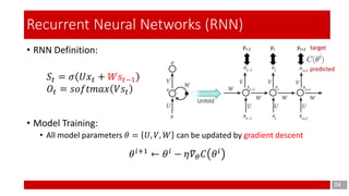
  • 4. • RNN Definition: • Model Training: • All model parameters 𝜃 = 𝑈, 𝑉, 𝑊 can be updated by gradient descent 04 Recurrent Neural Networks (RNN) 𝑆𝑡 = 𝜎 𝑈𝑥𝑡 + 𝑊𝑠𝑡−1 𝑂𝑡 = 𝑠𝑜𝑓𝑡𝑚𝑎𝑥 𝑉𝑠𝑡 𝜃 𝑖+1 ← 𝜃 𝑖 − 𝜂𝛻𝜃 𝐶 𝜃 𝑖
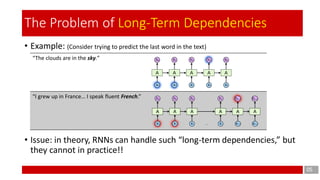
  • 5. • Example: (Consider trying to predict the last word in the text) • Issue: in theory, RNNs can handle such “long-term dependencies,” but they cannot in practice!! “The clouds are in the sky.” “I grew up in France… I speak fluent French.” 05 The Problem of Long-Term Dependencies
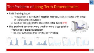
  • 6. • RNN Training Issue: (1) The gradient is a product of Jacobian matrices, each associated with a step in the forward computation (2) Multiply the same matrix at each time step during BPTT • The gradient becomes very small or very large quickly • Vanishing or Exploding gradient • The error surface is either very flat or very steep 06 The Problem of Long-Term Dependencies
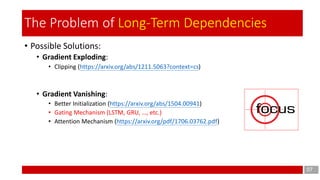
  • 7. • Possible Solutions: • Gradient Exploding: • Clipping (https://arxiv.org/abs/1211.5063?context=cs) • Gradient Vanishing: • Better Initialization (https://arxiv.org/abs/1504.00941) • Gating Mechanism (LSTM, GRU, …, etc.) • Attention Mechanism (https://arxiv.org/pdf/1706.03762.pdf) 07 The Problem of Long-Term Dependencies
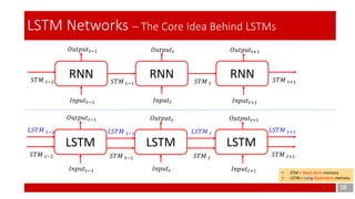
  • 8. 08 LSTM Networks – The Core Idea Behind LSTMs RNN RNNRNN 𝐼𝑛𝑝𝑢𝑡 𝑡 𝑂𝑢𝑡𝑝𝑢𝑡 𝑡 𝑆𝑇𝑀 𝑡−1 𝑆𝑇𝑀 𝑡 𝐼𝑛𝑝𝑢𝑡 𝑡−1 𝑂𝑢𝑡𝑝𝑢𝑡 𝑡−1 𝐼𝑛𝑝𝑢𝑡 𝑡+1 𝑂𝑢𝑡𝑝𝑢𝑡 𝑡+1 𝑆𝑇𝑀 𝑡−2 𝑆𝑇𝑀 𝑡+1 • STM = Short-term memory • LSTM = Long Short-term memory LSTM LSTMLSTM 𝐼𝑛𝑝𝑢𝑡 𝑡 𝑂𝑢𝑡𝑝𝑢𝑡 𝑡 𝑆𝑇𝑀 𝑡−1 𝑆𝑇𝑀 𝑡 𝐼𝑛𝑝𝑢𝑡 𝑡−1 𝑂𝑢𝑡𝑝𝑢𝑡 𝑡−1 𝐼𝑛𝑝𝑢𝑡 𝑡+1 𝑂𝑢𝑡𝑝𝑢𝑡 𝑡+1 𝑆𝑇𝑀 𝑡−2 𝑆𝑇𝑀 𝑡+1 𝐿𝑆𝑇𝑀 𝑡−1 𝐿𝑆𝑇𝑀 𝑡 𝐿𝑆𝑇𝑀 𝑡−2 𝐿𝑆𝑇𝑀 𝑡+1
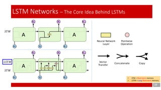
  • 9. 09 LSTM Networks – The Core Idea Behind LSTMs • STM = Short-term memory • LSTM = Long Short-term memory 𝐿𝑆𝑇𝑀 𝑆𝑇𝑀 𝑆𝑇𝑀
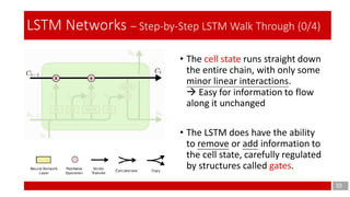
  • 10. 10 LSTM Networks – Step-by-Step LSTM Walk Through (0/4) • The cell state runs straight down the entire chain, with only some minor linear interactions.  Easy for information to flow along it unchanged • The LSTM does have the ability to remove or add information to the cell state, carefully regulated by structures called gates.
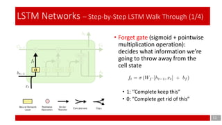
  • 11. 11 LSTM Networks – Step-by-Step LSTM Walk Through (1/4) • Forget gate (sigmoid + pointwise multiplication operation): decides what information we’re going to throw away from the cell state • 1: ‘’Complete keep this” • 0: “Complete get rid of this”
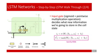
  • 12. 12 LSTM Networks – Step-by-Step LSTM Walk Through (2/4) • Input gate (sigmoid + pointwise multiplication operation): decides what new information we’re going to store in the cell state Vanilla RNN
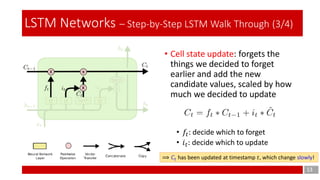
  • 13. 13 LSTM Networks – Step-by-Step LSTM Walk Through (3/4) • Cell state update: forgets the things we decided to forget earlier and add the new candidate values, scaled by how much we decided to update • 𝑓𝑡: decide which to forget • 𝑖 𝑡: decide which to update ⟹ 𝐶𝑡 has been updated at timestamp 𝑡, which change slowly!
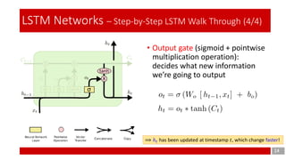
  • 14. 14 LSTM Networks – Step-by-Step LSTM Walk Through (4/4) • Output gate (sigmoid + pointwise multiplication operation): decides what new information we’re going to output ⟹ ℎ 𝑡 has been updated at timestamp 𝑡, which change faster!
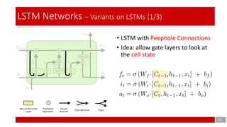
  • 15. 15 LSTM Networks – Variants on LSTMs (1/3) • LSTM with Peephole Connections • Idea: allow gate layers to look at the cell state
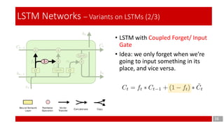
  • 16. 16 LSTM Networks – Variants on LSTMs (2/3) • LSTM with Coupled Forget/ Input Gate • Idea: we only forget when we’re going to input something in its place, and vice versa.
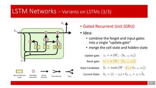
  • 17. 17 LSTM Networks – Variants on LSTMs (3/3) • Gated Recurrent Unit (GRU) • Idea: • combine the forget and input gates into a single “update gate” • merge the cell state and hidden state Update gate: Reset gate: State Candidate: Current State:
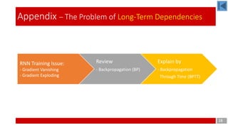
  • 18. Explain by - Backpropagation Through Time (BPTT) RNN Training Issue: - Gradient Vanishing - Gradient Exploding Review - Backpropagation (BP) 18 Appendix – The Problem of Long-Term Dependencies
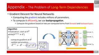
  • 19. 𝜕 𝐶 𝜃 𝜕 𝑤𝑖𝑗 𝑙 𝜕 𝐶 𝜃 𝜕 𝑤𝑖𝑗 𝑙 • Gradient Descent for Neural Networks • Computing the gradient includes millions of parameters. • To compute it efficiently, we use backpropagation. • Compute the gradient based on two pre-computed terms from forward and backward pass. 19 Appendix – The Problem of Long-Term Dependencies 𝜕 𝐶 𝜃 𝜕 𝑤𝑖𝑗 𝑙 BPTT BP
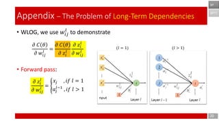
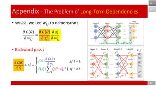
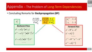
  • 20. 𝜕 𝐶 𝜃 𝜕 𝑤𝑖𝑗 𝑙 = 𝜕 𝐶 𝜃 𝜕 𝑧𝑖 𝑙 𝜕 𝑧𝑖 𝑙 𝜕 𝑤𝑖𝑗 𝑙 • WLOG, we use 𝑤𝑖𝑗 𝑙 to demonstrate • Forward pass: 20 Appendix – The Problem of Long-Term Dependencies 𝜕 𝑧𝑖 𝑙 𝜕 𝑤𝑖𝑗 𝑙 = ൝ 𝑥𝑗 , 𝑖𝑓 𝑙 = 1 𝑎𝑗 𝑙−1 , 𝑖𝑓 𝑙 > 1 (𝑙 = 1) (𝑙 > 1) BPTT BP
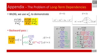
  • 21. 𝜕 𝐶 𝜃 𝜕 𝑤𝑖𝑗 𝑙 = 𝜕 𝐶 𝜃 𝜕 𝑧𝑖 𝑙 𝜕 𝑧𝑖 𝑙 𝜕 𝑤𝑖𝑗 𝑙 • WLOG, we use 𝑤𝑖𝑗 𝑙 to demonstrate • Backward pass : 21 Appendix – The Problem of Long-Term Dependencies (𝑙 = 𝐿) (𝑙 < 𝐿) 𝛿𝑖 𝐿 = 𝜕 𝐶 𝜃 𝜕 𝑧𝑖 𝐿 = 𝜕 𝐶 𝜃 𝜕 𝑦𝑖 𝜕 𝑦𝑖 𝜕 𝑧𝑖 𝐿 = 𝜕 𝐶 𝜃 𝜕 𝑦𝑖 𝜕𝑎𝑖 𝐿 𝜕 𝑧𝑖 𝐿 = 𝜕 𝐶 𝜃 𝜕 𝑦𝑖 𝜕σ 𝑧𝑖 𝐿 𝜕 𝑧𝑖 𝐿 = 𝜕 𝐶 𝜃 𝜕 𝑦𝑖 σ′ 𝑧𝑖 𝐿 BPTT BP 𝛿𝑖 𝑙 = 𝜕 𝐶 𝜃 𝜕 𝑧𝑖 𝑙 = ෍ 𝑘 𝜕 𝐶 𝜃 𝜕 𝑧 𝑘 𝑙+1 𝜕 𝑧 𝑘 𝑙+1 𝜕𝑎𝑖 𝐿 𝜕𝑎𝑖 𝐿 𝜕 𝑧𝑖 𝑙 = 𝜕𝑎𝑖 𝐿 𝜕 𝑧𝑖 𝑙 ෍ 𝑘 𝜕 𝐶 𝜃 𝜕 𝑧 𝑘 𝑙+1 𝜕 𝑧 𝑘 𝑙+1 𝜕𝑎𝑖 𝐿 = 𝜕𝑎𝑖 𝐿 𝜕 𝑧𝑖 𝑙 ෍ 𝑘 𝛿𝑖 𝑙+1 𝜕 𝑧 𝑘 𝑙+1 𝜕𝑎𝑖 𝐿 = σ′ 𝑧𝑖 𝑙 ෍ 𝑘 𝛿𝑖 𝑙+1 𝑤 𝑘𝑖 𝑙+1 𝜕 𝐶 𝜃 𝜕 𝑧𝑖 𝑙 ≜ 𝛿𝑖 𝑙 = σ′ 𝑧𝑖 𝐿 𝜕 𝐶 𝜃 𝜕 𝑦𝑖 , 𝑖𝑓 𝑙 = 𝐿 σ′ 𝑧𝑖 𝑙 ෍ 𝑘 𝛿𝑖 𝑙+1 𝑤 𝑘𝑖 𝑙+1 , 𝑖𝑓 𝑙 < 𝐿
  • 22. 𝜕 𝐶 𝜃 𝜕 𝑤𝑖𝑗 𝑙 = 𝜕 𝐶 𝜃 𝜕 𝑧𝑖 𝑙 𝜕 𝑧𝑖 𝑙 𝜕 𝑤𝑖𝑗 𝑙 • WLOG, we use 𝑤𝑖𝑗 𝑙 to demonstrate • Backward pass : 22 Appendix – The Problem of Long-Term Dependencies BPTT BP 𝜕 𝐶 𝜃 𝜕 𝑧𝑖 𝑙 ≜ 𝛿𝑖 𝑙 = σ′ 𝑧𝑖 𝐿 𝜕 𝐶 𝜃 𝜕 𝑦𝑖 , 𝑖𝑓 𝑙 = 𝐿 σ′ 𝑧𝑖 𝑙 ෍ 𝑘 𝛿𝑖 𝑙+1 𝑤 𝑘𝑖 𝑙+1 , 𝑖𝑓 𝑙 < 𝐿
  • 23. 𝜕 𝐶 𝜃 𝜕 𝑤𝑖𝑗 𝑙 = 𝜕 𝐶 𝜃 𝜕 𝑧𝑖 𝑙 𝜕 𝑧𝑖 𝑙 𝜕 𝑤𝑖𝑗 𝑙 • Concluding Remarks for Backpropagation (BP) 23 Appendix – The Problem of Long-Term Dependencies BPTT BP
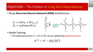
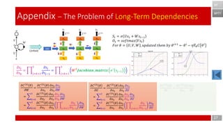
  • 24. • Recap Recurrent Neuron Network (RNN) Architectures • Model Training: • All model parameters 𝜃 = 𝑈, 𝑉, 𝑊 can be updated by gradient descent 24 Appendix – The Problem of Long-Term Dependencies BPTT BP 𝑆𝑡 = 𝜎 𝑈𝑥𝑡 + 𝑊𝑠𝑡−1 𝑂𝑡 = 𝑠𝑜𝑓𝑡𝑚𝑎𝑥 𝑉𝑠𝑡 𝜃 𝑖+1 ← 𝜃 𝑖 − 𝜂𝛻𝜃 𝐶 𝜃 𝑖
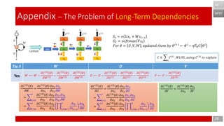
  • 25. 25 Appendix – The Problem of Long-Term Dependencies BPTT BP 𝑆𝑡 = 𝜎 𝑈𝑥 𝑡 + 𝑊𝑠𝑡−1 𝑂𝑡 = 𝑠𝑜𝑓𝑡𝑚𝑎𝑥 𝑉𝑠𝑡 𝐹𝑜𝑟 𝜃 = 𝑈, 𝑉, 𝑊 , 𝑢𝑝𝑑𝑎𝑡𝑒𝑑 𝑡ℎ𝑒𝑚 𝑏𝑦 𝜃 𝑖+1 ← 𝜃 𝑖 − 𝜂𝛻𝜃 𝐶 𝜃 𝑖 𝑾 𝑼 𝑽 𝑊(1) ⟵ 𝑊 1 − 𝜕𝐶 3 𝜃 𝜕𝑊 1 𝑊(2) ⟵ 𝑊 2 − 𝜕𝐶 3 𝜃 𝜕𝑊 2 𝑊(3) ⟵ 𝑊 3 − 𝜕𝐶 3 𝜃 𝜕𝑊 3 𝑈(1) ⟵ 𝑈 1 − 𝜕𝐶 3 𝜃 𝜕𝑈 1 𝑈(2) ⟵ 𝑈 2 − 𝜕𝐶 3 𝜃 𝜕𝑈 2 𝑈(3) ⟵ 𝑈 3 − 𝜕𝐶 3 𝜃 𝜕𝑈 3 𝑉(3) ⟵ 𝑉 3 − 𝜕𝐶 3 𝜃 𝜕𝑉 3 𝑊 ⟵ 𝑊 − 𝜕𝐶 3 𝜃 𝜕𝑊 1 − 𝜕𝐶 3 𝜃 𝜕𝑊 2 − 𝜕𝐶 3 𝜃 𝜕𝑊 3 𝑈 ⟵ 𝑈 − 𝜕𝐶 3 𝜃 𝜕𝑈 1 − 𝜕𝐶 3 𝜃 𝜕𝑈 2 − 𝜕𝐶 3 𝜃 𝜕𝑈 3 𝑉 ⟵ 𝑉 − 𝜕𝐶 3 𝜃 𝜕𝑉 3 𝐶 ≜ ෍ 𝑡 𝐶 𝑡 , 𝑊𝐿𝑂𝐺, 𝑢𝑠𝑖𝑛𝑔 𝐶 3 𝑡𝑜 𝑒𝑥𝑝𝑙𝑎𝑖𝑛 Tie 𝜃 NO Yes
  • 26. 26 Appendix – The Problem of Long-Term Dependencies BPTT BP 𝜕𝐶 3 𝜃 𝜕𝑊 = 𝜕𝐶 3 𝜃 𝜕𝑜3 𝜕𝑜3 𝜕𝑠3 𝜕𝑠3 𝜕𝑊 = ෍ 𝑘=0 3 𝜕𝐶 3 𝜃 𝜕𝑜3 𝜕𝑜3 𝜕𝑠3 𝜕𝑠3 𝜕𝑠 𝑘 𝜕𝑠 𝑘 𝜕𝑊 = ෍ 𝑘=0 3 𝜕𝐶 3 𝜃 𝜕𝑜3 𝜕𝑜3 𝜕𝑠3 ෑ 𝑗=𝑘+1 3 𝜕𝑠𝑗 𝜕𝑠𝑗−1 𝜕𝑠 𝑘 𝜕𝑊 𝑾 𝑼 𝑽 𝑊 ⟵ 𝑊 − 𝜕𝐶 3 𝜃 𝜕𝑊 1 − 𝜕𝐶 3 𝜃 𝜕𝑊 2 − 𝜕𝐶 3 𝜃 𝜕𝑊 3 𝑈 ⟵ 𝑈 − 𝜕𝐶 3 𝜃 𝜕𝑈 1 − 𝜕𝐶 3 𝜃 𝜕𝑈 2 − 𝜕𝐶 3 𝜃 𝜕𝑈 3 𝑉 ⟵ 𝑉 − 𝜕𝐶 3 𝜃 𝜕𝑉 3 Tie 𝜃 Yes 𝜕𝐶 3 𝜃 𝜕𝑈 = 𝜕𝐶 3 𝜃 𝜕𝑜3 𝜕𝑜3 𝜕𝑠3 𝜕𝑠3 𝜕𝑈 = ෍ 𝑘=1 3 𝜕𝐶 3 𝜃 𝜕𝑜3 𝜕𝑜3 𝜕𝑠3 𝜕𝑠3 𝜕𝑠 𝑘 𝜕𝑠 𝑘 𝜕𝑈 = ෍ 𝑘=1 3 𝜕𝐶 3 𝜃 𝜕𝑜3 𝜕𝑜3 𝜕𝑠3 ෑ 𝑗=𝑘+1 3 𝜕𝑠𝑗 𝜕𝑠𝑗−1 𝜕𝑠 𝑘 𝜕𝑈 𝜕𝐶 3 𝜃 𝜕𝑉 = 𝜕𝐶 3 𝜃 𝜕𝑜3 𝜕𝑜3 𝜕𝑉 𝐶 ≜ ෍ 𝑡 𝐶 𝑡 , 𝑊𝐿𝑂𝐺, 𝑢𝑠𝑖𝑛𝑔 𝐶 3 𝑡𝑜 𝑒𝑥𝑝𝑙𝑎𝑖𝑛 𝑆𝑡 = 𝜎 𝑈𝑥 𝑡 + 𝑊𝑠𝑡−1 𝑂𝑡 = 𝑠𝑜𝑓𝑡𝑚𝑎𝑥 𝑉𝑠𝑡 𝐹𝑜𝑟 𝜃 = 𝑈, 𝑉, 𝑊 , 𝑢𝑝𝑑𝑎𝑡𝑒𝑑 𝑡ℎ𝑒𝑚 𝑏𝑦 𝜃 𝑖+1 ← 𝜃 𝑖 − 𝜂𝛻𝜃 𝐶 𝜃 𝑖
  • 27. 27 Appendix – The Problem of Long-Term Dependencies BPTT BP 𝜕𝑠𝑗 𝜕𝑠 𝑘 = ෑ 𝑗=𝑘+1 3 𝜕𝑠𝑗 𝜕𝑠𝑗−1 = ෑ 𝑗=𝑘+1 3 𝑊 𝑇 𝑱𝒂𝒄𝒐𝒃𝒊𝒂𝒏_𝒎𝒂𝒕𝒓𝒊𝒙 𝜎′ 𝑠𝑗−1 𝜕𝐶 3 𝜃 𝜕𝑊 = 𝜕𝐶 3 𝜃 𝜕𝑜3 𝜕𝑜3 𝜕𝑠3 𝜕𝑠3 𝜕𝑊 = ෍ 𝑘=0 3 𝜕𝐶 3 𝜃 𝜕𝑜3 𝜕𝑜3 𝜕𝑠3 𝜕𝑠3 𝜕𝑠 𝑘 𝜕𝑠 𝑘 𝜕𝑊 = ෍ 𝑘=0 3 𝜕𝐶 3 𝜃 𝜕𝑜3 𝜕𝑜3 𝜕𝑠3 ෑ 𝑗=𝑘+1 3 𝜕𝑠𝑗 𝜕𝑠𝑗−1 𝜕𝑠 𝑘 𝜕𝑊 𝜕𝐶 3 𝜃 𝜕𝑈 = 𝜕𝐶 3 𝜃 𝜕𝑜3 𝜕𝑜3 𝜕𝑠3 𝜕𝑠3 𝜕𝑈 = ෍ 𝑘=1 3 𝜕𝐶 3 𝜃 𝜕𝑜3 𝜕𝑜3 𝜕𝑠3 𝜕𝑠3 𝜕𝑠 𝑘 𝜕𝑠 𝑘 𝜕𝑈 = ෍ 𝑘=1 3 𝜕𝐶 3 𝜃 𝜕𝑜3 𝜕𝑜3 𝜕𝑠3 ෑ 𝑗=𝑘+1 3 𝜕𝑠𝑗 𝜕𝑠𝑗−1 𝜕𝑠 𝑘 𝜕𝑈 𝜕𝐶 3 𝜃 𝜕𝑉 = 𝜕𝐶 3 𝜃 𝜕𝑜3 𝜕𝑜3 𝜕𝑉 𝑆𝑡 = 𝜎 𝑈𝑥 𝑡 + 𝑊𝑠𝑡−1 𝑂𝑡 = 𝑠𝑜𝑓𝑡𝑚𝑎𝑥 𝑉𝑠𝑡 𝐹𝑜𝑟 𝜃 = 𝑈, 𝑉, 𝑊 , 𝑢𝑝𝑑𝑎𝑡𝑒𝑑 𝑡ℎ𝑒𝑚 𝑏𝑦 𝜃 𝑖+1 ← 𝜃 𝑖 − 𝜂𝛻𝜃 𝐶 𝜃 𝑖
  • 28. • Understand the difficulty of training recurrent neural networks • Gradient Exploding • Gradient Vanishing • One possible solution for solving the gradient vanishing problem is “Gating mechanism”, which is the key concept of LSTM • LSTM can be “deep” if we stack multiple LSTM cells • Extensions: • Uni-directional v.s. Bi-directional • One-to-one, One-to-many, Many-to-one, Many-to-Many (w/ or w/o Encoder-Decoder) 28 Conclusions
  • 29. • Understanding LSTM Networks http://colah.github.io/posts/2015-08-Understanding-LSTMs/ • Prof. Hung-yi Lee Courses https://www.youtube.com/watch?v=xCGidAeyS4M https://www.youtube.com/watch?v=rTqmWlnwz_0 • On the difficulty of training recurrent neural networks https://arxiv.org/abs/1211.5063 • UDACITY Courses: Intro to Deep Learning with PyTorch https://classroom.udacity.com/courses/ud188 29 References
  • 30. 20 Thanks for your listening.