Materi 10 - Penelitian Pemodelan Komputer.pdf
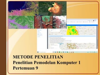
- 1. METODE PENELITIAN Penelitian Pemodelan Komputer 1 Pertemuan 9
- 2. 2 ◼ A mathematical model is central to most computational scientific research. ◼ Other terms often used in connection with mathematical modeling are • Computer modeling • Computer simulation • Computational mathematics • Scientific Computation • Mathematic Modeling Computer Modeling & Simulation
- 3. 3 1. Creates a mathematical representation of some phenomenon to better understand it. 2. Matches observation with symbolic representation. 3. Informs theory and explanation. The success of a mathematical model depends on how easily it can be used, and how accurately it predicts and how well it explains the phenomenon being studied. Computer Modeling & Simulation
- 4. Computer Simulations ◼Computer simulation is the process of making a computer behave the same as ...whatever it is we are interested in. • Atoms • Cooling metal alloy • A society of voters • Climate change • A galaxy 4
- 5. Computer Simulations ◼Simulations have applications across a range of disciplines: ◼Physics – solids, gases, fluids, solar systems ◼Chemistry – molecular dynamics ◼Biology – gene networks, predator-prey populations ◼Sociology – socio networks, opinion propagation ◼Technology – internet traffic, local networks ◼Management – queuing, workflow models ◼Finance & Economics – stock markets, supply- demand ◼Agriculture – pest outbreak, rainy or drought season 5
- 6. Computer Simulations ◼Computer simulations allow us to observe the behaviour of these systems at (relatively) low cost. ◼Other methods of investigating these systems may involve complicated theoretical research or experimental research with potentially expensive equipment. 6
- 7. Computer Simulations There are some definitions of simulations: ◼"The representation of the dynamic behaviour of the system by moving it from state to state in accordance with well-defined operating rules." – A. Alan B. Pritsker (1984) ◼"We can therefore define simulation as the technique of solving problems by the observation of the performance, over the time, of a dynamic model of the system." – Bernard P. Zeigler (1976) ◼"A simulation is a method for implementing a model." – Defense Acquisition University 7
- 8. Computer Simulations ◼To create a computer simulation to approximate a system, a model of that system must first be made. These are most often mathematical models. ◼"A model is a description of some system intended to predict what happens if certain actions are taken" – Bratley, Bennet & Schrage (1987) 8
- 9. Models ◼Modelling is a large discipline in itself and creating a system requires a lot of mathematical ability and understanding of the system. ◼Models are usually composed of variables and relationships between them. Exactly what these variables represent and what the relationships between them are can vary. 9
- 10. Models The variables of the model must represent the state of the system. The state is split into different components to represent the different parts of the system. These are sometimes called model components. For example: A car in a traffic simulator may have a position, a size and a velocity. 10
- 11. Models When using computer simulations, it is important to understand the limitations of the model you are using. A simulation (no matter how accurate) cannot provide useful results if the model is not suitable for the system you are studying. A model is considered valid if the system it describes sufficiently near to the real system. 11
- 12. What is Simulation? A Simulation of a system is the operation of a model, which is a representation of that system. The model is amenable to manipulation which would be impossible, too expensive, or too impractical to perform on the system which it portrays. The operation of the model can be studied, and, from this, properties concerning the behavior of the actual system can be inferred.
- 13. Applications: 1. Designing and analyzing manufacturing systems 2. Evaluating H/W and S/W requirements for a computer system 3. Evaluating a new military weapons system or tactics 4. Determining ordering policies for an inventory system 5. Designing communications systems and message protocols for them
- 14. Applications:(continued) Designing and operating transportation facilities such as freeways, airports, subways, or ports Evaluating designs for service organizations such as hospitals, post offices, or fast-food restaurants Analyzing financial or economic systems
- 15. Perbedaan : ◼A model • An abstraction of the system being studied that we claim behaves much like the original ◼Computer simulation • A physical system is modeled as a set of mathematical equations and/or algorithmic procedures
- 16. Perbedaan : ◼ Computer simulation (continued) • Model is translated into a high-level language and executed on the Von Neumann computer ◼ Computational models • Also called simulation models • Used to –Design new systems –Study and improve the behavior of existing systems
- 17. Computational models (continued) • Allow the use of an interactive design methodology (sometimes called computational steering) • Used in most branches of science and engineering
- 18. Using a Simulation in an Interactive Design Environment
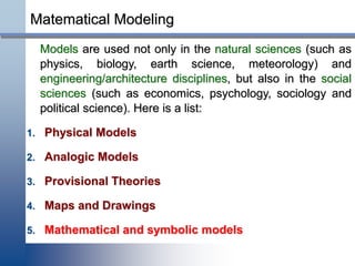
- 19. Matematical Modeling Models are used not only in the natural sciences (such as physics, biology, earth science, meteorology) and engineering/architecture disciplines, but also in the social sciences (such as economics, psychology, sociology and political science). Here is a list: 1. Physical Models 2. Analogic Models 3. Provisional Theories 4. Maps and Drawings 5. Mathematical and symbolic models
- 20. MATHEMATICAL MODELING Definitions A mathematical model is a representation, in mathematical terms, of certain aspects of a non- mathematical system. A mathematical model is a set of mathematical equations that are intended to capture the effect of certain system variables on certain other system variables. A model may be prescriptive or illustrative, but, above all, it must be useful !
- 21. A mathematical model is a description of a system using mathematical concepts and language. The process of developing a mathematical model is termed mathematical modelling. Mathematical models are used not only in the natural sciences (such as physics, biology, earth science, meteorology) and engineering disciplines (e.g. computer science, artificial intelligence), but also in the social sciences (such as economics, psychology, sociology and political science); physicists, engineers, statisticians, operations research analysts and economists use mathematical models most extensively. A mathematical model usually describes a system by a set of variables and a set of equations that establish relationships between the variables.
- 22. WHY MATH MODELING FOR PROCESS SYSTEMS? ◼ Understand the problem: Why does one need a model? ◼ Is it: ➢to design a controller? ➢to analyze the performance of the process? ➢to understand the process better? ➢to simplify the complexity of a system ➢etc.
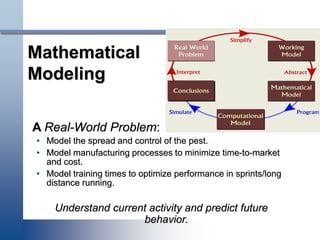
- 24. Mathematical Modeling A Real-World Problem: • Model the spread and control of the pest. • Model manufacturing processes to minimize time-to-market and cost. • Model training times to optimize performance in sprints/long distance running. Understand current activity and predict future behavior.
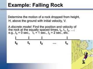
- 25. Example: Falling Rock Determine the motion of a rock dropped from height, H, above the ground with initial velocity, V. A discrete model: Find the position and velocity of the rock at the equally spaced times, t0, t1, t2, …; e.g., t0 = 0 sec., t1 = 1 sec., t2 = 2 sec., etc. |______|______|____________|______ t0 t1 t2 … tn
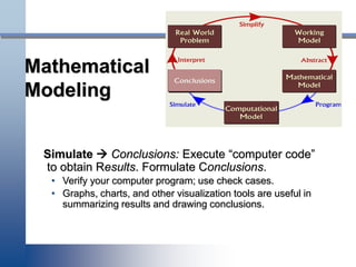
- 26. Mathematical Modeling Simplify → Working Model: Identify and select factors that describe important aspects of the Real World Problem; deter- mine those factors that can be neglected. • Determine governing principles, physical laws. • Identify model variables; focus on how they are related. • State simplifying assumptions.
- 27. Example: Falling Rock ◼ Governing principles: d = v*t and v = a*t. ◼ Simplifying assumptions: • Gravity is the only force acting on the body. • Flat earth. • No drag (air resistance). • Rock’s position and velocity above the ground will be modeled at discrete times (t0, t1, t2, …) until rock hits the ground.
- 28. Mathematical Modeling Abstract → Mathematical Model: Express the Working Model in mathematical terms; write down mathematical equations whose solution describes the Working Model. There may not be a "best" model; the one to be used will depend on the questions to be studied.
- 29. Example: Falling Rock v0 v1 v2 … vn x0 x1 x2 … xn |______|______|____________|______ t0 t1 t2 … tn t0 = 0; x0 = H; v0 = V; Δt = ti+1 - ti t1= t0 + Δt x1= x0 + (v0*Δt) v1= v0 - (g*Δt) t2= t1 + Δt x2= x1 + (v1*Δt) v2= v1 - (g*Δt) …
- 30. Mathematical Modeling Program → Computational Model: Implement Mathematical Model in “computer code”. If model is simple enough, it may be solved analytically; otherwise, a computer program is required.
- 31. Example: Falling Rock Pseudo Code Input V, initial velocity; H, initial height g, acceleration due to gravity Δt, time step; imax, maximum number of steps Output ti, t-value at time step i xi, height at time ti vi, velocity at time ti
- 32. Example: Falling Rock Initialize ti = t0 = 0; vi = v0 = V; xi = x0 = H print ti, xi, vi Time stepping: i = 1, imax ti = ti + Δt xi = xi - vi*Δt vi = vi + g*Δt print ti, xi, vi if (xi <= 0), xi = 0; quit
- 33. Mathematical Modeling Simulate → Conclusions: Execute “computer code” to obtain Results. Formulate Conclusions. • Verify your computer program; use check cases. • Graphs, charts, and other visualization tools are useful in summarizing results and drawing conclusions.
- 34. Mathematical Modeling Interpret Conclusions and compare with Real World Problem behavior. • If model results do not “agree” with physical reality or experimental data, reexamine the Working Model and repeat modeling steps. • Usually, modeling process proceeds through several iterations until model is“acceptable”.
- 35. Example: Falling Rock To create a more more realistic model of a falling rock, some of the simplifying assumptions could be dropped: • Incorporate air resistance, depends on shape of rock. • Improve discrete model: approximate velocities in the midpoint of time intervals instead of the beginning. • Reduce the size of Δt.
- 37. Daftar Pustaka ◼ Mathematical Modeling, Summer Teacher Institute, 2002
- 38. Questions?
- 39. ANOVA
- 40. TERIMA KASIH
