MATLAB-Introd.ppt

MATLAB Endalkachew Teshome (Dr) 1
)
( 2
2
y
x
xe
z 


An Introduction to
MATLAB
Compiled By: Endalkachew Teshome
(PhD)
Department of Mathematics,
AMU, 2022

1. MATLAB Basics
2. Graphs :
2D /3D Plotting
3. Programming in MATLAB
Main Content:
)
( 2
2
y
x
xe
z 



MATLAB
Endalkachew Teshome (Dr)
3
1. MATLAB Basics
MATLAB is a general-purpose mathematical software
It is particularly suitable for doing numerical
computations with matrices and vectors.
( MATLAB : Matrix Laboratory )
It is possible to write computer programs in
MATLAB and implement it to solve problems of
interest.
It can also display information graphically.

MATLAB Endalkachew Teshome (Dr 4
Getting Started
• To bring up MATLAB from the operating system you should
- Double click on the matlab icon (MATLAB Logo)
(If the software is installed on your computer).
• This will present the MATLAB command window with prompt
>>
If this appeared, you are in MATLAB window.
• To exit out of the MATLAB use one of the following commands
>> exit or >> quit

• You can perform arithmetic operations ( +, - , *, / , ^ )
as in a calculator and more. For instance, see
>> 5+2 , 5-2, 5*2, 5/2 , 5^2,
• Brackets , ( ), manage the order of operation as usual . Exa:
>> ( (5+3)^2 – (2*2) ) / 6 (ans = 10)
Arithmetic Operations
• Complex numbers: MATLAB knows that . . Exa.:
1


i
>> (5+3i) – (2 – i) (ans = 3 + 4i )
>> i *(5+3i) (ans = –3 + 5i )
>> (10+15i) / (3+4i) (ans = 3.6 + 0.2i )
• Two type of division: / = right division ; = left division
>> 4/2 , 24, (ans = 2, 0.50 )

Format: Set output format, i.e., the way numbers appear
• format short 4 digits after decimal point.
• format long 14 digits after decimal point.
• format bank 2 digits after decimal point
• format rat Approximation by ratio of integers (fraction).
• format Default. Same as short.
Examples
>> format short ;
>> 1/2, 2/3, (ans = 0.5000, 0.6667
>> format long; 1/2, 2/3 (ans = 0.50000000000000
0.66666666666667
>> format bank; 1/2, 2/3 ( ans = 0.50, 0.67 )
>> format rat ; 1/2, 2/3 (ans = 1/2, 2/3 )
>> (10 + 15i) / (3+4i) (ans = 18/5 + 1/5 i )
>> format (switch to the default format - short)

MATLAB Endalkachew Teshome (Dr 7
Built-in functions
• MATLAB contains several built-in functions such as,
sqrt, sin, cos, exp, log, abs etc.
• Example: Consider the following
>> sqrt(9) , sin(pi/2), exp(1), log( exp(2) ) , abs(-5)
( ans = 3 , 1, 2.7183, 2, 5 )
• To see the list of more built-in elementary functions , type
>> help elfun
• For a list of other special functions , type
>> help specfun
For instance: rem, floor, ceil, round, etc.
For instance: factor, gcd, lcm, factorial, etc.

>> b = 11
b =
11
• MATLAB is case sensitive. That is, for instance, a and A are
different things for MATLAB
Variables and assignment
• A variable, such as x, x0, x_1, a, etc, is a storage object
(container) of a value. For instance, consider the following
>> a = 5
a =
5
>> c= a^2 + b ( you get c = 36 )
>> c= sqrt(a+b) ( you get c = 4 )
• Note that the previous value of c is replaced (overwritten)
• You can free (empty) a variable , say b, holding a value by the command
>> clear b
• If you want to free all the variables that hold values, use the command
>> clear

Vectors
a row vector
A column vector
To extract i-th
component of vector
x, type x(i)
To extract i to j
components of vector
x, type x(i:j)
)
1
5
2
1
(

x
1
5
3
A
 
 
  




Matlab Syntax
>> x = [1 2 5 1]
x =
1 2 5 1
>> A = [1; 5; 3]
A =
1
5
3
>> x3= x(3)
x3 =
5
>> a= x(2:3)
a =
2
5

MATLAB
)
Endalkachew Teshome (Dr 10
Matrix
Transpose
B = AT












1
2
3
4
1
5
3
2
1
A
Matlab Syntax
>> A = [1 2 3;
5 1 4;
3 2 -1]
A =
1 2 3
5 1 4
3 2 -1
>> B = A’
B =
1 5 3
2 1 2
3 4 -1
>> A_ij= A(1,2)
A_ij=
5
i-j entry of matrix A
A_ij = A(i,j)

Extract
i-th row of A
Ai= A(i,:)
j-th column of A
Aj= A(:,j)
Matlab Syntax
>> A2 = A(2,:)
A2 =
5 1 4
>> A3 = A(:,3)
A3 =
3
2
-1
>> d= diag(A)
d=
1
1
-1
Diagonal of A
d = diag(A)

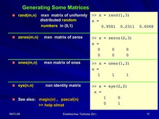
Generating Some Matrices
rand(m,n) mxn matrix of uniformly
distributed random
numbers in (0,1)
zeros(m,n) mxn matrix of zeros
ones(m,n) mxn matrix of ones
eye(n,n) nxn identity matrix
See also: magic(n) , pascal(n)
>> help elmat
>> x = rand(1,3)
x =
0.9501 0.2311 0.6068
>> x = zeros(2,3)
x =
0 0 0
0 0 0
>> x = ones(1,3)
x =
1 1 1
>> x = eye(2,2)
x =
1 0
0 1

MATLAB Berhanu G (Dr) 13
• You can add, multiply, etc, given matrices A and B. Just write
A+B, A*B, c*A, when c is a constant, etc.
The following are more MatLab commands for a given matrix A:
det(A) determinant of A
inv(A) inverse of A
D = eig(A) vector D containing the eigenvalues of A
[ V,D] = eig(A) matrix V whose columns are eigenvectors of A &
diagonal matrix D of corresponding eigenvalues
length(A) number of columns of A
rank(A) rank of A
Result
Command

length(x) number of elements (components) of x
norm(x) vector norm , ||x||
sum(x) sum of its elements
max(x) largest element of x
min(x) smallest element of x
mean(x) average or mean value
sort(x) sort (list) in ascending order
Given a vector x the following commands are useful:
dot(A,B) Scalar product of A and B.
cross(A,B) vector product of A and B (both in 3-dim)
scalar and vector product of two vectors A & B:
Example: Consider >> A= [ 6, -3, 9, 5 ]; B= [ 3, 2, 5, 0 ]
>> c=dot(A,B) ( c = 57 )
>> m= max(A) ( m= 9)
>> [m,i] = max(A) ( m= 9, i=3) i.e., 2nd variable i is the index of max element

Vectors/ Matrix can be input of built-in functions in which case
evaluation is performed component-wise. For instance,
Consider >> x= [ 6, pi, 25, 0]
>> A= [ 4, 25, 0;
1, 16, 2]
Then,
>> a = sqrt(x) , b= sqrt(A)
a =
2.4495 1.7725 5.0000 0
b =
2.0000 5.0000 0
1.0000 4.0000 1.4142
See also,
>> sin(x) , sin(A)

+ addition : As usual A+B ( Also k+A for kR )
– subtraction : As usual A – B (Also A–k for kR )
* Multiplication : As usual A*B, (Also k*A for kR )
/ right division : A/B = A*inv(B) , (if B is invertible)
left division : AB = inv(A)*B , (if A is invertible)
^ power : A^2 = A*A ( A square matrix)
Operations on Vectors / Matrices A, B
.* Element-by-element Multiplication A.*B
./ Element-by-element right division A./B
.^ Element-by-element power A.^n
Example: Consider >> A= [ 6, 12, 10]; B= [ 3, 2, 5 ]
>> A .* B ans= [18 24 50 ]
>> A ./ B ans= [ 2 6 2 ]
>> A .^ B ans= [216 144 100000]

Generating Arrays/Vectors
One can define an array with a particular
structure using the command:
a : step : b
If step is not given, Matlab takes 1 for it.
>> x = 1:0.5:3
x =
1 1.5 2 2.5 3
>> x = -2:4
x =
-2 -1 0 1 2 4
linspace(a, b, n) generates a row vector of n equally spaced
points between a and b.
Example: >> x=linspace(1,10,4) ( x = [ 1, 4, 7, 10 ] )
linspace(a, b) generates a row vector of 100 equally spaced
points between a and b.

Solution of System of Linear Equations Ax = b
• You need only to remember : det(A) 0  x = A–1b
• So, to solve a system of nxn linear equations Ax = b :
 enter the coefficient matrix A, column vector b,
and check for det(A)
 The command
x = inv(A)*b
produces the solution.

Creating Functions
• A Script is simply a file containing the sequence of MATLAB commands
which we wish to execute to define a function or to solve a task at hand.
That is, Script is a computer program written in the language of MATLAB.
This can be done by constructing m-file (MATLAB file) in the m-file Editor:
>> edit
• To define your own function, the first line of the script has the form
function output = function_name( input arguments )
• Example: To define the function f(x) = x2+1 as an m-file :
Type in the m- Editor
function f = myfun1(x)
f = x.^2 +1 ;
and save it as myfun1

• Once the script of the function is saved in m-file named myfun1.m, you
can use it like the built-in functions to compute. For instance,
>> myfun1( 2)
ans =
5
>> z= myfun1(2)+3 (ans = 8)
• Built-in function quad(‘ f ’, a, b ) produces numerical integration
(definite integral) of f(x) from a to b.
i.e., quad(‘ f ’, a, b ) =
>> I=quad('myfun1', 0, 1)
I =
1.3333
• See the effect of : >> x = [-2,-1,0,1,2]; myfun1( x)
( )
b
a
f x dx


• You can define also a function of several variables.
• For instance, for f(x,y) = x2 + y2 , you may define
function f = myfun2(X)
x=X(1); y=X(2)
f = x .^2 + y .^2  4*x ;
• Once this is saved as, say, myfun2.m, you can use it like any
built in function. For example, see:
myfun2([0, 1]) , v = 10*myfun2([0, 1])

I. 2-D Plotting
>> x = 0: 0.01 : 2*pi;
y = sin(x);
plot(x,y, ‘r’),
• You can choose the color of the graph:
grid on
2. Graphs
>> x = 0: 0.01: 2*pi;
y = sin(x);
plot(x,y)
xlabel('x = 0: pi/2 ' )
ylabel('Sine of x' )
title('Plot of the Sine
Function')

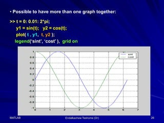
>> t = 0: 0.01: 2*pi;
y1 = sin(t); y2 = cos(t);
plot( t , y1, t, y2 );
legend(‘sint’, ‘cost’ ), grid on
• Possible to have more than one graph together:

2. Programming in MATLAB :
• MATLAB is also a Programming Language. So, you can write
your own MATLAB program to solve a specific problem.
• By creating a script file with the extension .m you can write and
run a program just like a user defined function.
• Once you wrote a program in the MATLAB language and saved it
as m-file, say, myfile.m, then you can run the program by typing
myfile at the MATLB command window in the same way as any
other function; i.e.,
>> myfile
2.1 Basics in MATLAB Programming

• In particular, if a MATLAB program is required to take an external
input and return an output , you should begin the script (on the
first line) with the following format :
function output = Program_name(input)
• The output and input can be vector or scalar as desired.
• For example, the following is a MATLAB program that takes certain real
numbers x1, x2, …, xn as in put vector X; and returns two vector out puts
Y and Z, where components Y are square root of x1, x2, …, xn,
and components Z are square of x1, x2, …, xn, respectively.
function [Y, Z ] = prog1(X)
% This program is saved in prog1.m
% Comment ( or note) line starts with percentage notation
Y=sqrt(X);
Z=X.^2;
• After saving this, say as prog1.m, you can run it just like a function:
>> x=[0, 4, 9, 16 ]; [y,z]=prog1(x)

• MATLAB program may not necessarily begin as a function if its
input is fixed and included in the internal part of the program.
For example, the following program does the same as prog1.n
when the input is fixed, say x= [9, 15, 20, 25].
% Program name prog2.m
% This program finds the square root and square of
% of the components of x= [0, 4, 9, 16];
x = [0, 4, 9, 16];
y=sqrt(x);
z=x.^2;
fprintf(' Square Root: y=(%3.4f, %3.4f, %3.4f, %3.4f) n', y );
fprintf(' Square : z=(%5.0f, %5.0f, %5.0f, %5.0f) n', z );
Note: fprintf writes formatted data:
• Here, a format %n.mf means, the output can have up to n digits
before decimal point and m digits after decimal point.
• n is the line termination character (new line follows).
• See also disp

• Program in MATLAB consists of a sequence of MATLAB commands
and may includes the following important flow control commands.
I: Conditional
if <condition1>
commands
elseif <condition2>
commands
else
commands
end
2.2 Conditional Statements and Loops
== equal
~= not equal
< less than
<= less than or equal
> greater than
>= greater than or equal
Logical Operations:
& AND
| OR
~ NOT
Relational Operations:

Roots of a quadratic equation:
Consider a quadratic equation
ax2 + bx +c =0 .
Write a Matlab program that
• takes any real number a, b, c as input
• checks the sign of the discriminant of the quadratic equation and
tells whether it has two real roots, one real root or complex root
• finds the roots of the quadratic equation and returns the roots in
r1 and r2
Example

function rootquad(a,b,c)
% Finds the root of quadratic function f(x) = ax^2 + bx + c
D = b^2 - 4*a*c; % D is its discriminant
if (D > 0)
r1 = (-b + sqrt(D)) / (2*a); r2 = (-b - sqrt(D)) / (2*a);
r=[r1, r2];
disp( ‘ It has two real roots: ‘ ), r
elseif (D==0)
r = – b /(2*a);
disp( ‘ It has one double root: ‘ ), r
else
r1 = (-b + sqrt(D)) / (2*a) ;
r2 = r1' ;
r=[r1, r2];
disp( ‘ Has No real Root. Its complex roots are: ‘ ) , r
end

• For and While loops
For loop:
for index = initial:step:termial
commands
end
The actions of these flow control commands (loops) are similar
to that of any other common programming languages.
While loop:
while <condition>
commands
end
II. Loops:

• This executes a statement or group of statements a
predetermined number of times. function z= zsum(n)
s=0;
for i = 1:n
s = s + i^2;
end
z=s;
I. The for loop:
for index = initial:step:termial
commands /statements
end
disp(' n z(n) ' )
disp('---------------')
for n = 1:10
s=0;
for i = 1:n
s = s + i^2;
end
fprintf('%2.0f %6.0f n', n,s);
end
• For instance, the following loop computes
• You can nest for loops.
For example, the following program
computes
and print out the result for each
natural number n =1 to 10.
for a given number n.
2
1
( )
n
i
z n i

 
2
1
( )
n
i
z n i

 

• While loop repeats statements an indefinite number of times.
• The statements are executed while the given expression is true.
• For instance, write a MATLAB program for the following:
Given a number x1 > 1, find a sequence x1, x2, x3, …, xn such that
that xi+1= ½ xi and xi 1 for all i.
II. The while loop:
While <expression>
statements
end
function half(x1)
i=1; x(1)=x1;
while x(i) >= 2 %To get half of x(i) if it is >=2
x(i+1) = 0.5*x(i);
i=i+1;
end
disp( ‘The desired sequence is: ’), x
Note: While and for loops can be nested in one another, if needed.

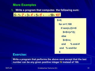
1. Write a program that computes the following sum:
2 2 2 2
2 4 6 1
3 .
0
1 5 9
9 0
S        
S=0;
for n=1:100
if rem(n,2)==0
S=S+(n^2);
else
S=S+n;
end % end-if
end % end-for
S
Write a program that performs the above sum except that the last
number can be any given positive integer N instead of 100.
Exercise:
More Examples

2. Bisection Method : To solve f(x)=0 on [a, b], say 2
( ) 5
x
f x xe x
  
function bisect(a,b,tol)
f=inline('x*exp(x) + x^2 - 5 ');
iter=0; c=(a+b)*0.5; err=abs(b-a)*0.5;
disp(' iter a b c=(a+b)/2 f(c) ')
disp('----------------------------------------------------')
if f(a)* f(b)>0
disp(' The method cannot be applied f(a)f(b)>0')
return % the program terminates
end
while (err>tol)
fprintf('%2.0f %10.4f %10.4f %10.6f %10.6f n', iter, a, b, c, f(c))
if f(a)*f(c)<0
b=c;
else
a=c;
end % end-if
iter=iter+1;
c=(a+b)*0.5;
err=abs(b-a)*0.5;
end %end-while

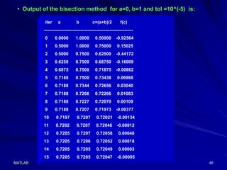
MATLAB Berhanu G (Dr) 46
iter a b c=(a+b)/2 f(c)
-------------------------------------------------------------
0 0.0000 1.0000 0.50000 -0.92564
1 0.5000 1.0000 0.75000 0.15025
2 0.5000 0.7500 0.62500 -0.44172
3 0.6250 0.7500 0.68750 -0.16009
4 0.6875 0.7500 0.71875 -0.00862
5 0.7188 0.7500 0.73438 0.06988
6 0.7188 0.7344 0.72656 0.03040
7 0.7188 0.7266 0.72266 0.01083
8 0.7188 0.7227 0.72070 0.00109
9 0.7188 0.7207 0.71973 -0.00377
10 0.7197 0.7207 0.72021 -0.00134
11 0.7202 0.7207 0.72046 -0.00012
12 0.7205 0.7207 0.72058 0.00048
13 0.7205 0.7206 0.72052 0.00018
14 0.7205 0.7205 0.72049 0.00003
15 0.7205 0.7205 0.72047 -0.00005
• Output of the bisection method for a=0, b=1 and tol =10^(-5) is:

3. Newton’s Method
• Newton’s method is faster to find a root of function, if it is applicable
• Given a differentiable function f(x) and an initial guess x1, the method
tries to construct the sequence of points, xn , which “converge to
a root” of the function using the recursive relation
)
(
'
)
(
1 n
n
x
f
x
f
n
n x
x 


• The value of f is zero at its root.
• In computation, however, we may approximate a root by some r, where
| f(r) | <  , for some sufficiently small  , say,  = 10-12.
• For instance, let us consider a Matlab program that approximates a
root of
x
x
e
x
f x


  2
)
(
in [ -1, 1 ] , starting from x1 = 0.

% script name newton.m
% Newton’s method to find approximate root of f(x)= exp(-x)-x^2-x
f = inline( ' exp(-x)-x^2-x ' );
df=inline(' -exp(-x)-2*x-1 ' ); %df is derivative of f
x(1)=0; % initial guess
n=1;
disp('_______________________________________')
disp(' iter x f(x) ' )
disp('_______________________________________')
fprintf('%2.0f %12.6f %12.12f n', n ,x(n),f(x(n)) )
while ( abs(f(x(n))) > 10^(-12))& (n<100)
x(n+1)= x(n) - ( f(x(n)) / df(x(n)) );
n=n+1;
fprintf('%2.0f %12.6f %12.12f n', n ,x(n),f(x(n)) )
end
fprintf('The approximate root is x= %8.5f n', x(n) )

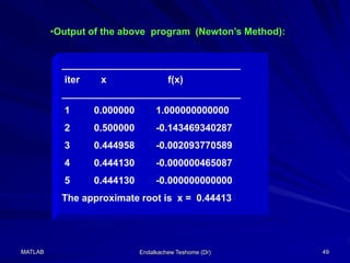
•Output of the above program (Newton’s Method):
_________________________________
iter x f(x)
_________________________________
1 0.000000 1.000000000000
2 0.500000 -0.143469340287
3 0.444958 -0.002093770589
4 0.444130 -0.000000465087
5 0.444130 -0.000000000000
The approximate root is x = 0.44413

MATLAB-Introd.ppt

More Related Content

MATLAB-Introd.ppt