Location via proxy:   [ UP ]  
[Report a bug]   [Manage cookies]                
SlideShare a Scribd company logo

1

MBA 532 Business Statistics   by  Rushan Abeygunawardana Department of Statistics, University of Colombo

2

Introduction A time series is a collection of observations made sequentially in time.  In economics and business Share price on successive days Export total in successive months, Yearly sales figures  Weekly bank interest rates In meteorology Daily rainfall, daily temperature Hourly wind speed In demography Population of a country in successive years In marketing Sales in successive months The purposes of time series analysis are; To understand or model the behavior of the observed series. To predict or forecast future of a series based on the past values of the series.

3

Continuous and Discrete Time Series A time series is said to be  continuous  when observations are made continuously in time. The term “continuous’ is used for series of this type even when the measured variable  can only take  a discrete set of values.  A time series is said to  discrete  when observations are taken only at specific times, usually equally spaced. The term “discrete” is used for series of this type even when the measured variable is a continuous variable.

4

Continuous and Discrete Time Series In the discrete time series the observations are usually taken at equally intervals. Discrete time series can arise in several ways. Sampled: Read off (or digitize) a continuous time series model with the values at equal interval of time. Aggregate (accumulate) : E.g.: monthly exports, weekly rainfall The special feature of time series analysis is the fact that successive observations are usually  not  independent and that the analysis must taken into account the  time order  of the observations. When successive observations are dependent the future values may be forecast form the past data.

5

Deterministic Time Series and Stochastic Time Series Deterministic Time Series If a time series can be forecast exactly, it is said to be deterministic time series. Stochastic Time Series For stochastic time series the exact prediction is impossible and must be replaced by the idea that future values have a probability distribution which is conditioned by knowledge of the past values.

6

Objectives of Time Series Analysis There are several possible objectives in time series analysis and these objectives may be classified as; Description Explanation Forecasting Control

7

Objectives of Time Series Analysis Description In the time series analysis the first step is plot the data and obtained simple descriptive measures of the main properties of the series. (i.e. tread, seasonal variations, outliers, turning points etc.) In the plot of the raw sales data; There are upward trends  There are downward trends There are turning points For some series, the variation is dominated by such “obvious” features (trend and seasonal variation) and a fairly simple model may be perfectly adequate. For some other series, more advance techniques will be required. And more complex models (such as various types of stochastic process) are required to describe the series.

8

Objectives of Time Series Analysis Explanation When observations are taken on two or more variables, it may be possible to use the variation in one series to explain the variation in the other series. To see how see level is affected by temperature and pressure To see how sales are affected by price and economic conditions To see how sales of soft drink varies with the daily temperature A stochastic model is fitted and then forecast the future values and then input process is adjusted so as to keep the process on target.

9

Objectives of Time Series Analysis Forecasting (Predicting) Given an observed time series, one may want to predict the future values of the series. Forecasting is vary important task in the analysis of economic and industrial time series.

10

Objectives of Time Series Analysis Control When a time series is generated, which measure the “quality” of a manufacturing process, the aim of analysis may be to control the process. Control processes are of several different kinds. In quality control, observations are plotted on a control chart and controller takes actions using pattern of the graph.

11

Types of variations Traditional models of time series analysis are mainly concerned with decomposing the variation in a series into; Trend Seasonal variation Cyclic variation Irregular variation  Trend (T) This is defined as “long term change in mean”. Trend measured the average change in the variable per unit time. It shows the graduate and general pattern of development, which is often described by a straight line or some type of smooth curve. When speaking of a trend, we must take into account the number of observations available and make subjective assessment of what is long term trend.

12

Types of variations Seasonal variation (S) Many time series exhibits variation which is  annual in period . This variation arises due to the seasonal factors. This yearly variation is easy to understand and we shall see that is can be measured explicitly and /or removed from the data to give de-seasonalized data. Sales of school stationeries in December and January Sales of charismas trees

13

Types of variations Cyclic variation Apart from the seasonal effects, sometimes series shows variation at a fixed period of time due to some another physical causes. Daily variation in temperature Cyclic variation is characterized by recurring up and down movements which are different form seasonal fluctuations in that they extend over longer / shorter period of time, usually two or more years or less than one year.

14

Types of variations Irregular variation After trend and cyclic variation has been removed from a set of data, we are left with a series of residuals, which may or may not be “random”. Then we may see some anther type of variation which do not show a regular pattern and it is called the irregular variation. We shall examine various techniques for analyzing series of this type to see if some of the appropriate irregular variation may be explained in terms of probability models such as Moving Average (MA) or Autoregressive (AR) models which will be discussed later.

15

Stationary Time Series This is a time series with; No systematic change in mean (No trend) No systematic change in variation (No seasonal variation) No strictly periodic variation (No cyclic variation). Most of the probability theory (stochastic process) of time series is concerned with stationary time series and for this reason time series analysis often requires one to turn a non-stationary into a stationary one so as to use these theories. That is, it may be interested of remove the trend and seasonal variation from a set of data and then try to model the variation in residuals by means of stationary stochastic process.

16

Time Plot This is the first step in analyzing a time series data. That is plot the observations against time. The time plot shows whether and how the values in a dataset change over time. You can make a time plot of any numeric data.  Time Plot graphs are similar to X-Y graphs, and are used to display time-value data pairs. A Time Plot data item consists of two data values—the time and the value—which translate into the x and y coordinate, respectively. Each data item is displayed as a symbol, but you can add a line, bubbles, or fill areas to better delineate the data. Because of the nature of the coordinate system, Time Plot graphs do not have categories. Time graphs are good for graphing the values at irregular intervals, such as sampling data at random times. Plotting a time series is not a easy task. The choice of scales, the size of the intercept, and the way that the points are plotted (continuous lines or separate points) may substantially affected the way the plot “look” and so the analyst must examine very carefully and make the judgments.

17

Common Approaches to Forecasting Used when historical data are unavailable Considered highly subjective and judgmental Common Approaches to Forecasting Causal Quantitative forecasting methods Qualitative forecasting methods Time Series Use past data to predict future values

18

Common Approaches to Forecasting… Quantitative forecasting methods can be used when:  Past information about the variable being forecast is available,  The information can be quantified, and  It can be assumed that the pattern of the past will continue into the future In such cases, a forecast can be developed using a time series method or a causal method: Time series methods: The historical data are restricted to past values of the variable. The objective is to discover a pattern in the historical data and then extrapolate the pattern into the future. Ex.: trend analysis, classical decomposition, moving averages, exponential smoothing, ARIMA. Causal forecasting methods: Based on the assumption that the variable we are forecasting has a cause-effect relationship with one or more other variables (e.g.: the sales volume can be influenced by advertising expenditures). Ex.: regression analysis. Qualitative methods generally involve the use of expert judgment to develop forecasts.

19

Traditional Models in Time Series Analysis A procedure for dealing with a time series is to fit a suitable model to the data. There are three commonly use time series. Additive models Multiplicative models A combination of 1 and 2

20

Smoothing the Time Series Calculate moving averages to get an overall impression of the pattern of movement over time Moving Average:  averages of consecutive time series values for a chosen period of length L A series of arithmetic means over time Result dependent upon choice of L (length of period for computing means) Example :  Five-year moving average  First average: Second average:

21

Example: Moving Average Method 23 40 25 27 32 48 33 37 37 50 40 1 2 3 4 5 6 7 8 9 10 11  Sales Year

22

Calculating Moving Averages Each moving average is for a consecutive block of 5 years 40 50 37 37 33 48 32 27 25 40 23 Sales 11 10 9 8 7 6 5 4 3 2 1 Year 9 8 7 6 5 4 3 Average Year 5-Year Moving Average 39.4 41.0 37.4 35.4 33.0 34.4 29.4

23

Exponential Smoothing A   weighted moving average Weights decline exponentially Most recent observation weighted most Used for smoothing and short term forecasting (often one period into the future) The weight (smoothing coefficient) is W Subjectively chosen Range from 0 to 1 Smaller W gives more smoothing, larger W gives less smoothing The weight is: Close to 0 for smoothing out unwanted cyclical and irregular components Close to 1 for forecasting

24

Exponential Smoothing Model Exponential smoothing model where: E i  = exponentially smoothed value for period i E i-1  = exponentially smoothed value already   computed for period i - 1   Y i  = observed value in period i   W = weight (smoothing coefficient), 0 < W < 1 For i = 2, 3, 4, …

25

Exponential Smoothing Example Suppose we use weight W = 0.2 E 1  = Y 1  since no prior information exists -- 23 26.4 26.12 26.296 27.437 31.549 31.840 32.872 33.697 etc. Forecast from prior period (E i-1 ) 23 40 25 27 32 48 33 37 37 50 etc. Sales (Y i ) 23 (.2)(40)+(.8)(23)=26.4 (.2)(25)+(.8)(26.4)=26.12 (.2)(27)+(.8)(26.12)=26.296 (.2)(32)+(.8)(26.296)=27.437 (.2)(48)+(.8)(27.437)=31.549 (.2)(48)+(.8)(31.549)=31.840 (.2)(33)+(.8)(31.840)=32.872 (.2)(37)+(.8)(32.872)=33.697 (.2)(50)+(.8)(33.697)=36.958 etc. Exponentially Smoothed Value for this period (E i ) 1 2 3 4 5 6 7 8 9 10 etc. Time Period (i)

26

Sales vs. Smoothed Sales Fluctuations have been smoothed The smoothed value in this case is generally a little low, since the trend is upward sloping and the weighting factor is only .2

27

Trend-Based Forecasting Forecast for time period 6: 20 40 30 50 70 65 ?? 0 1 2 3 4 5 6 1999 2000 2001 2002 2003 2004 2005 Sales (y) Time Period (X) Year

28

Introduction to ARIMA models The Autoregressive Integrated Moving Average (ARIMA) models, or Box-Jenkins methodology, are a class of linear models that is capable of representing stationary as well as non-stationary time series. ARIMA models rely heavily on autocorrelation patterns in data.  Both ACF and PACF are used to select an initial model. The Box-Jenkins methodology uses an iterative approach: An initial model is selected, from a general class of ARIMA models, based on an examination of the TS and an examination of its autocorrelations for several time lags. The chosen model is then checked against the historical data to see whether it accurately describes the series: the model fits well if the residuals are generally small, randomly distributed, and contain no useful information. If the specified model is not satisfactory, the process is repeated using a new model designed to improve on the original one.  Once a satisfactory model is found, it can be used for forecasting.

29

Autoregressive Models AR(p) An AR(p) model is a  regression model with lagged values  of the dependent variable in the independent variable positions, hence the name  autoregressive  model. A  p th-order autoregressive model, or AR(p), takes the form: Autoregressive models are appropriate for stationary time series, and the coefficient  Ф 0   is related to the constant level of the series.

30

AR(p) Theoretical behavior of the ACF and PACF for AR(1) and AR(2) models: ACF    0 PACF = 0 for lag > 2 AR(2) ACF    0 PACF = 0 for lag > 1 AR(1)

31

Moving Average Models MA(q) MA(q) model is a regression model with the dependent variable,  Yt, depending on previous values of the errors  rather than on the variable itself.  A  q th-order moving average model, or MA(q), takes the form: MA models are appropriate for stationary time series. The weights  ω i  do  not necessarily sum to 1 and may be positive or negative.

32

MA(q) Theoretical behavior of the ACF and PACF for MA(1) and MA(2) models: MA(2) ACF = 0 for lag > 2;  PACF    0 MA(1) ACF = 0 for lag > 1;  PACF    0

33

ARMA(p,q) Models A model with autoregressive terms can be combined with a model having moving average terms to get an ARMA(p,q) model: ARMA(p,q) models can describe a wide variety of behaviors for stationary time series. Theoretical behavior of the ACF and PACF for autoregressive-moving average processes: Note  that: ARMA(p,0) = AR(p) ARMA(0,q) = MA(q) In practice, the values of p and q each  rarely exceed 2 . In this context… “ Die out”  means “tend to zero gradually” “ Cut off”  means “disappear” or “is zero” ACF PACF AR(p) Die out Cut off after the order p of the process MA(q) Cut off after the order q of the process Die out ARMA(p,q) Die out Die out

34

Example: Fitting an ARIMA Model The series show an  upward trend . The first several autocorrelations are persistently large and trailed off to zero rather slowly    a  trend  exists and this time series is  nonstationary  (it does not vary about a fixed level) Idea: to  difference  the data to see if we could eliminate the trend and create a stationary series.

35

Example: Fitting an ARIMA Model… A plot of the differenced data appears to vary about a fixed level. Comparing the autocorrelations with their error limits, the only  significant  autocorrelation is at lag 1. Similarly, only the lag 1 partial autocorrelation is significant. The  PACF  appears to  cut off  after lag 1, indicating  AR(1)  behavior. The  ACF  appears to  cut off  after lag 1, indicating  MA(1)  behavior    we will try:  ARIMA(1,1,0)  and  ARIMA(0,1,1) A  constant term  in each model will be included to allow for the fact that the series of differences appears to vary about a level greater than zero.

36

Example: Fitting an ARIMA Model… The  LBQ statistics  are not significant as indicated by the large p-values for either model.  ARIMA(1,1,0) ARIMA(0,1,1)

37

Example: Fitting an ARIMA Model… Finally, there is  no significant residual autocorrelation  for the ARIMA(1,1,0) model. The results for the ARIMA(0,1,1) are similar.  Therefore, either model is  adequate  and provide nearly the same one-step-ahead forecasts.

38

The first sample  ACF  coefficient is significantly different form zero. The autocorrelation at lag 2 is close to significant and opposite in sign from the lag 1 autocorrelation. The remaining autocorrelations are small. This suggests either an  AR(1)  model or an  MA(2)  model. The first  PACF  coefficient is significantly different from zero, but none of the other partial autocorrelations approaches significance, This suggests an  AR(1)  or  ARIMA(1,0,0) ARIMA The time series of readings appears to vary about a fixed level of around 80, and the autocorrelations die out rapidly toward zero    the time series seems to be  stationary .

39

Both models appear to fit the data well. The estimated  coefficients  are significantly different from zero and the mean square ( MS ) errors are similar. ARIMA AR(1) = ARIMA(1,0,0) MA(2) = ARIMA(0,0,2) A  constant term  is included in both models to allow for the fact that the readings vary about a level other than zero. Let’s take a look at the  residuals ACF …

40

ARIMA Finally, there is  no significant residual autocorrelation  for the ARIMA(1,0,0) model. The results for the ARIMA(0,0,2) are similar.  Therefore, either model is  adequate  and provide nearly the same three-step-ahead forecasts. Since the AR(1) model has two parameters (including the constant term) and the MA(2) model has three parameters, applying the  principle of parsimony  we would use the simpler  AR(1)  model to forecast future readings.

41

Building an ARIMA model The first step in model identification is to determine whether the series is stationary. It is useful to look at a plot of the series along with the sample ACF. If the series is not stationary, it can often be converted to a stationary series by differencing: the original series is replaced by a series of differences and an ARMA model is then specified for the differenced series (in effect, the analyst is modeling changes rather than levels) Models for nonstationary series are called Autoregressive Integrated Moving Average models, or ARIMA(p,d,q), where d indicates the amount of differencing. Once a stationary series has been obtained, the analyst must identify the form of the model to be used by comparing the sample ACF and PACF to the theoretical ACF and PACF for the various ARIMA models. Principle of parsimony: “all things being equal, simple models are preferred to complex models” Once a tentative model has been selected, the parameters for that model are estimated using least squares estimates.

42

Building an ARIMA model … Before using the model for forecasting, it must be checked for adequacy. Basically, a model is adequate if the residuals cannot be used to improve the forecasts, i.e.,  The residuals should be random and normally distributed The individual residual autocorrelations should be small. Significant residual autocorrelations at low lags or seasonal lags suggest the model is inadequate After an adequate model has been found, forecasts can be made. Prediction intervals based on the forecasts can also be constructed. As more data become available, it is a good idea to monitor the forecast errors, since the model must need to be reevaluated if: The magnitudes of the most recent errors tend to be consistently larger than previous errors, or  The recent forecast errors tend to be consistently positive or negative Seasonal ARIMA (SARIMA) models contain: Regular AR and MA terms that account for the correlation at low lags Seasonal AR and MA terms that account for the correlation at the seasonal lags

43

Introduction to ARIMA models

44

The End Rushan A B Abeygunawardana  Thursday, December 1, 2011

More Related Content

Mba 532 2011_part_3_time_series_analysis

  • 1. MBA 532 Business Statistics by Rushan Abeygunawardana Department of Statistics, University of Colombo
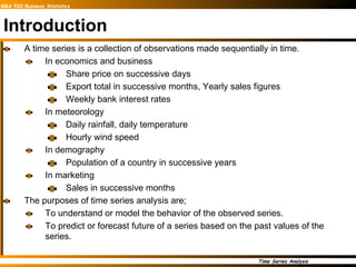
  • 2. Introduction A time series is a collection of observations made sequentially in time. In economics and business Share price on successive days Export total in successive months, Yearly sales figures Weekly bank interest rates In meteorology Daily rainfall, daily temperature Hourly wind speed In demography Population of a country in successive years In marketing Sales in successive months The purposes of time series analysis are; To understand or model the behavior of the observed series. To predict or forecast future of a series based on the past values of the series.
  • 3. Continuous and Discrete Time Series A time series is said to be continuous when observations are made continuously in time. The term “continuous’ is used for series of this type even when the measured variable can only take a discrete set of values. A time series is said to discrete when observations are taken only at specific times, usually equally spaced. The term “discrete” is used for series of this type even when the measured variable is a continuous variable.
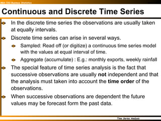
  • 4. Continuous and Discrete Time Series In the discrete time series the observations are usually taken at equally intervals. Discrete time series can arise in several ways. Sampled: Read off (or digitize) a continuous time series model with the values at equal interval of time. Aggregate (accumulate) : E.g.: monthly exports, weekly rainfall The special feature of time series analysis is the fact that successive observations are usually not independent and that the analysis must taken into account the time order of the observations. When successive observations are dependent the future values may be forecast form the past data.
  • 5. Deterministic Time Series and Stochastic Time Series Deterministic Time Series If a time series can be forecast exactly, it is said to be deterministic time series. Stochastic Time Series For stochastic time series the exact prediction is impossible and must be replaced by the idea that future values have a probability distribution which is conditioned by knowledge of the past values.
  • 6. Objectives of Time Series Analysis There are several possible objectives in time series analysis and these objectives may be classified as; Description Explanation Forecasting Control
  • 7. Objectives of Time Series Analysis Description In the time series analysis the first step is plot the data and obtained simple descriptive measures of the main properties of the series. (i.e. tread, seasonal variations, outliers, turning points etc.) In the plot of the raw sales data; There are upward trends There are downward trends There are turning points For some series, the variation is dominated by such “obvious” features (trend and seasonal variation) and a fairly simple model may be perfectly adequate. For some other series, more advance techniques will be required. And more complex models (such as various types of stochastic process) are required to describe the series.
  • 8. Objectives of Time Series Analysis Explanation When observations are taken on two or more variables, it may be possible to use the variation in one series to explain the variation in the other series. To see how see level is affected by temperature and pressure To see how sales are affected by price and economic conditions To see how sales of soft drink varies with the daily temperature A stochastic model is fitted and then forecast the future values and then input process is adjusted so as to keep the process on target.
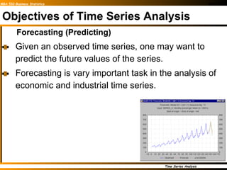
  • 9. Objectives of Time Series Analysis Forecasting (Predicting) Given an observed time series, one may want to predict the future values of the series. Forecasting is vary important task in the analysis of economic and industrial time series.
  • 10. Objectives of Time Series Analysis Control When a time series is generated, which measure the “quality” of a manufacturing process, the aim of analysis may be to control the process. Control processes are of several different kinds. In quality control, observations are plotted on a control chart and controller takes actions using pattern of the graph.
  • 11. Types of variations Traditional models of time series analysis are mainly concerned with decomposing the variation in a series into; Trend Seasonal variation Cyclic variation Irregular variation Trend (T) This is defined as “long term change in mean”. Trend measured the average change in the variable per unit time. It shows the graduate and general pattern of development, which is often described by a straight line or some type of smooth curve. When speaking of a trend, we must take into account the number of observations available and make subjective assessment of what is long term trend.
  • 12. Types of variations Seasonal variation (S) Many time series exhibits variation which is annual in period . This variation arises due to the seasonal factors. This yearly variation is easy to understand and we shall see that is can be measured explicitly and /or removed from the data to give de-seasonalized data. Sales of school stationeries in December and January Sales of charismas trees
  • 13. Types of variations Cyclic variation Apart from the seasonal effects, sometimes series shows variation at a fixed period of time due to some another physical causes. Daily variation in temperature Cyclic variation is characterized by recurring up and down movements which are different form seasonal fluctuations in that they extend over longer / shorter period of time, usually two or more years or less than one year.
  • 14. Types of variations Irregular variation After trend and cyclic variation has been removed from a set of data, we are left with a series of residuals, which may or may not be “random”. Then we may see some anther type of variation which do not show a regular pattern and it is called the irregular variation. We shall examine various techniques for analyzing series of this type to see if some of the appropriate irregular variation may be explained in terms of probability models such as Moving Average (MA) or Autoregressive (AR) models which will be discussed later.
  • 15. Stationary Time Series This is a time series with; No systematic change in mean (No trend) No systematic change in variation (No seasonal variation) No strictly periodic variation (No cyclic variation). Most of the probability theory (stochastic process) of time series is concerned with stationary time series and for this reason time series analysis often requires one to turn a non-stationary into a stationary one so as to use these theories. That is, it may be interested of remove the trend and seasonal variation from a set of data and then try to model the variation in residuals by means of stationary stochastic process.
  • 16. Time Plot This is the first step in analyzing a time series data. That is plot the observations against time. The time plot shows whether and how the values in a dataset change over time. You can make a time plot of any numeric data. Time Plot graphs are similar to X-Y graphs, and are used to display time-value data pairs. A Time Plot data item consists of two data values—the time and the value—which translate into the x and y coordinate, respectively. Each data item is displayed as a symbol, but you can add a line, bubbles, or fill areas to better delineate the data. Because of the nature of the coordinate system, Time Plot graphs do not have categories. Time graphs are good for graphing the values at irregular intervals, such as sampling data at random times. Plotting a time series is not a easy task. The choice of scales, the size of the intercept, and the way that the points are plotted (continuous lines or separate points) may substantially affected the way the plot “look” and so the analyst must examine very carefully and make the judgments.
  • 17. Common Approaches to Forecasting Used when historical data are unavailable Considered highly subjective and judgmental Common Approaches to Forecasting Causal Quantitative forecasting methods Qualitative forecasting methods Time Series Use past data to predict future values
  • 18. Common Approaches to Forecasting… Quantitative forecasting methods can be used when: Past information about the variable being forecast is available, The information can be quantified, and It can be assumed that the pattern of the past will continue into the future In such cases, a forecast can be developed using a time series method or a causal method: Time series methods: The historical data are restricted to past values of the variable. The objective is to discover a pattern in the historical data and then extrapolate the pattern into the future. Ex.: trend analysis, classical decomposition, moving averages, exponential smoothing, ARIMA. Causal forecasting methods: Based on the assumption that the variable we are forecasting has a cause-effect relationship with one or more other variables (e.g.: the sales volume can be influenced by advertising expenditures). Ex.: regression analysis. Qualitative methods generally involve the use of expert judgment to develop forecasts.
  • 19. Traditional Models in Time Series Analysis A procedure for dealing with a time series is to fit a suitable model to the data. There are three commonly use time series. Additive models Multiplicative models A combination of 1 and 2
  • 20. Smoothing the Time Series Calculate moving averages to get an overall impression of the pattern of movement over time Moving Average: averages of consecutive time series values for a chosen period of length L A series of arithmetic means over time Result dependent upon choice of L (length of period for computing means) Example : Five-year moving average First average: Second average:
  • 21. Example: Moving Average Method 23 40 25 27 32 48 33 37 37 50 40 1 2 3 4 5 6 7 8 9 10 11 Sales Year
  • 22. Calculating Moving Averages Each moving average is for a consecutive block of 5 years 40 50 37 37 33 48 32 27 25 40 23 Sales 11 10 9 8 7 6 5 4 3 2 1 Year 9 8 7 6 5 4 3 Average Year 5-Year Moving Average 39.4 41.0 37.4 35.4 33.0 34.4 29.4
  • 23. Exponential Smoothing A weighted moving average Weights decline exponentially Most recent observation weighted most Used for smoothing and short term forecasting (often one period into the future) The weight (smoothing coefficient) is W Subjectively chosen Range from 0 to 1 Smaller W gives more smoothing, larger W gives less smoothing The weight is: Close to 0 for smoothing out unwanted cyclical and irregular components Close to 1 for forecasting
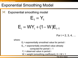
  • 24. Exponential Smoothing Model Exponential smoothing model where: E i = exponentially smoothed value for period i E i-1 = exponentially smoothed value already computed for period i - 1 Y i = observed value in period i W = weight (smoothing coefficient), 0 < W < 1 For i = 2, 3, 4, …
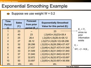
  • 25. Exponential Smoothing Example Suppose we use weight W = 0.2 E 1 = Y 1 since no prior information exists -- 23 26.4 26.12 26.296 27.437 31.549 31.840 32.872 33.697 etc. Forecast from prior period (E i-1 ) 23 40 25 27 32 48 33 37 37 50 etc. Sales (Y i ) 23 (.2)(40)+(.8)(23)=26.4 (.2)(25)+(.8)(26.4)=26.12 (.2)(27)+(.8)(26.12)=26.296 (.2)(32)+(.8)(26.296)=27.437 (.2)(48)+(.8)(27.437)=31.549 (.2)(48)+(.8)(31.549)=31.840 (.2)(33)+(.8)(31.840)=32.872 (.2)(37)+(.8)(32.872)=33.697 (.2)(50)+(.8)(33.697)=36.958 etc. Exponentially Smoothed Value for this period (E i ) 1 2 3 4 5 6 7 8 9 10 etc. Time Period (i)
  • 26. Sales vs. Smoothed Sales Fluctuations have been smoothed The smoothed value in this case is generally a little low, since the trend is upward sloping and the weighting factor is only .2
  • 27. Trend-Based Forecasting Forecast for time period 6: 20 40 30 50 70 65 ?? 0 1 2 3 4 5 6 1999 2000 2001 2002 2003 2004 2005 Sales (y) Time Period (X) Year
  • 28. Introduction to ARIMA models The Autoregressive Integrated Moving Average (ARIMA) models, or Box-Jenkins methodology, are a class of linear models that is capable of representing stationary as well as non-stationary time series. ARIMA models rely heavily on autocorrelation patterns in data. Both ACF and PACF are used to select an initial model. The Box-Jenkins methodology uses an iterative approach: An initial model is selected, from a general class of ARIMA models, based on an examination of the TS and an examination of its autocorrelations for several time lags. The chosen model is then checked against the historical data to see whether it accurately describes the series: the model fits well if the residuals are generally small, randomly distributed, and contain no useful information. If the specified model is not satisfactory, the process is repeated using a new model designed to improve on the original one. Once a satisfactory model is found, it can be used for forecasting.
  • 29. Autoregressive Models AR(p) An AR(p) model is a regression model with lagged values of the dependent variable in the independent variable positions, hence the name autoregressive model. A p th-order autoregressive model, or AR(p), takes the form: Autoregressive models are appropriate for stationary time series, and the coefficient Ф 0 is related to the constant level of the series.
  • 30. AR(p) Theoretical behavior of the ACF and PACF for AR(1) and AR(2) models: ACF  0 PACF = 0 for lag > 2 AR(2) ACF  0 PACF = 0 for lag > 1 AR(1)
  • 31. Moving Average Models MA(q) MA(q) model is a regression model with the dependent variable, Yt, depending on previous values of the errors rather than on the variable itself. A q th-order moving average model, or MA(q), takes the form: MA models are appropriate for stationary time series. The weights ω i do not necessarily sum to 1 and may be positive or negative.
  • 32. MA(q) Theoretical behavior of the ACF and PACF for MA(1) and MA(2) models: MA(2) ACF = 0 for lag > 2; PACF  0 MA(1) ACF = 0 for lag > 1; PACF  0
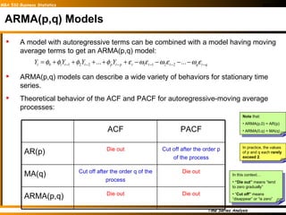
  • 33. ARMA(p,q) Models A model with autoregressive terms can be combined with a model having moving average terms to get an ARMA(p,q) model: ARMA(p,q) models can describe a wide variety of behaviors for stationary time series. Theoretical behavior of the ACF and PACF for autoregressive-moving average processes: Note that: ARMA(p,0) = AR(p) ARMA(0,q) = MA(q) In practice, the values of p and q each rarely exceed 2 . In this context… “ Die out” means “tend to zero gradually” “ Cut off” means “disappear” or “is zero” ACF PACF AR(p) Die out Cut off after the order p of the process MA(q) Cut off after the order q of the process Die out ARMA(p,q) Die out Die out
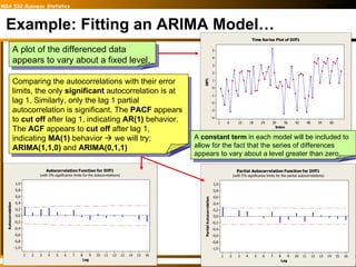
  • 34. Example: Fitting an ARIMA Model The series show an upward trend . The first several autocorrelations are persistently large and trailed off to zero rather slowly  a trend exists and this time series is nonstationary (it does not vary about a fixed level) Idea: to difference the data to see if we could eliminate the trend and create a stationary series.
  • 35. Example: Fitting an ARIMA Model… A plot of the differenced data appears to vary about a fixed level. Comparing the autocorrelations with their error limits, the only significant autocorrelation is at lag 1. Similarly, only the lag 1 partial autocorrelation is significant. The PACF appears to cut off after lag 1, indicating AR(1) behavior. The ACF appears to cut off after lag 1, indicating MA(1) behavior  we will try: ARIMA(1,1,0) and ARIMA(0,1,1) A constant term in each model will be included to allow for the fact that the series of differences appears to vary about a level greater than zero.
  • 36. Example: Fitting an ARIMA Model… The LBQ statistics are not significant as indicated by the large p-values for either model. ARIMA(1,1,0) ARIMA(0,1,1)
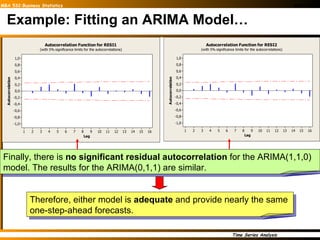
  • 37. Example: Fitting an ARIMA Model… Finally, there is no significant residual autocorrelation for the ARIMA(1,1,0) model. The results for the ARIMA(0,1,1) are similar. Therefore, either model is adequate and provide nearly the same one-step-ahead forecasts.
  • 38. The first sample ACF coefficient is significantly different form zero. The autocorrelation at lag 2 is close to significant and opposite in sign from the lag 1 autocorrelation. The remaining autocorrelations are small. This suggests either an AR(1) model or an MA(2) model. The first PACF coefficient is significantly different from zero, but none of the other partial autocorrelations approaches significance, This suggests an AR(1) or ARIMA(1,0,0) ARIMA The time series of readings appears to vary about a fixed level of around 80, and the autocorrelations die out rapidly toward zero  the time series seems to be stationary .
  • 39. Both models appear to fit the data well. The estimated coefficients are significantly different from zero and the mean square ( MS ) errors are similar. ARIMA AR(1) = ARIMA(1,0,0) MA(2) = ARIMA(0,0,2) A constant term is included in both models to allow for the fact that the readings vary about a level other than zero. Let’s take a look at the residuals ACF …
  • 40. ARIMA Finally, there is no significant residual autocorrelation for the ARIMA(1,0,0) model. The results for the ARIMA(0,0,2) are similar. Therefore, either model is adequate and provide nearly the same three-step-ahead forecasts. Since the AR(1) model has two parameters (including the constant term) and the MA(2) model has three parameters, applying the principle of parsimony we would use the simpler AR(1) model to forecast future readings.
  • 41. Building an ARIMA model The first step in model identification is to determine whether the series is stationary. It is useful to look at a plot of the series along with the sample ACF. If the series is not stationary, it can often be converted to a stationary series by differencing: the original series is replaced by a series of differences and an ARMA model is then specified for the differenced series (in effect, the analyst is modeling changes rather than levels) Models for nonstationary series are called Autoregressive Integrated Moving Average models, or ARIMA(p,d,q), where d indicates the amount of differencing. Once a stationary series has been obtained, the analyst must identify the form of the model to be used by comparing the sample ACF and PACF to the theoretical ACF and PACF for the various ARIMA models. Principle of parsimony: “all things being equal, simple models are preferred to complex models” Once a tentative model has been selected, the parameters for that model are estimated using least squares estimates.
  • 42. Building an ARIMA model … Before using the model for forecasting, it must be checked for adequacy. Basically, a model is adequate if the residuals cannot be used to improve the forecasts, i.e., The residuals should be random and normally distributed The individual residual autocorrelations should be small. Significant residual autocorrelations at low lags or seasonal lags suggest the model is inadequate After an adequate model has been found, forecasts can be made. Prediction intervals based on the forecasts can also be constructed. As more data become available, it is a good idea to monitor the forecast errors, since the model must need to be reevaluated if: The magnitudes of the most recent errors tend to be consistently larger than previous errors, or The recent forecast errors tend to be consistently positive or negative Seasonal ARIMA (SARIMA) models contain: Regular AR and MA terms that account for the correlation at low lags Seasonal AR and MA terms that account for the correlation at the seasonal lags
  • 44. The End Rushan A B Abeygunawardana Thursday, December 1, 2011